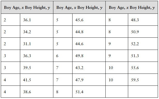
[DATA] The following data represent the height (inches) of boys between the ages of 2 and 10 years.
d. Assuming the residuals are normally distributed, construct a 95% confidence interval for the slope of the true least-squares regression line.
Verified step by step guidance
1
Step 1: Calculate the least-squares regression line for the data, which has the form \(\hat{y} = b_0 + b_1 x\), where \(b_1\) is the slope and \(b_0\) is the intercept. Use the formulas for slope and intercept:
\(b_1 = \frac{S_{xy}}{S_{xx}}\)
where
\(S_{xy} = \sum (x_i - \bar{x})(y_i - \bar{y})\) and
\(S_{xx} = \sum (x_i - \bar{x})^2\)
and
\(b_0 = \bar{y} - b_1 \bar{x}\)
Here, \(\bar{x}\) and \(\bar{y}\) are the sample means of \(x\) and \(y\) respectively.
Step 2: Calculate the residual standard error (standard deviation of residuals), \(s\), which measures the typical distance that the observed values fall from the regression line. Use the formula:
\(s = \sqrt{\frac{1}{n-2} \sum (y_i - \hat{y}_i)^2}\)
where \(n\) is the number of data points, \(y_i\) are observed values, and \(\hat{y}_i\) are predicted values from the regression line.
Step 3: Calculate the standard error of the slope, \(SE_{b_1}\), which quantifies the variability of the slope estimate. Use the formula:
\(SE_{b_1} = \frac{s}{\sqrt{S_{xx}}}\)
where \(s\) is the residual standard error from Step 2 and \(S_{xx}\) is from Step 1.
Step 4: Determine the critical value \(t^*\) from the \(t\)-distribution for a 95% confidence interval with \(n-2\) degrees of freedom. This value corresponds to the two-tailed 95% confidence level.
Step 5: Construct the 95% confidence interval for the slope \(b_1\) using the formula:
\(\left( b_1 - t^* \times SE_{b_1}, \quad b_1 + t^* \times SE_{b_1} \right)\)
This interval estimates the range in which the true slope of the population regression line lies with 95% confidence.
Verified video answer for a similar problem:
This video solution was recommended by our tutors as helpful for the problem above
Video duration:
5m
Play a video:
0 Comments
Key Concepts
Here are the essential concepts you must grasp in order to answer the question correctly.
Least-Squares Regression Line
The least-squares regression line is a straight line that best fits the data by minimizing the sum of the squared differences between observed and predicted values. It models the relationship between an independent variable (boy age) and a dependent variable (boy height), allowing predictions and interpretation of the slope and intercept.
Residuals are the differences between observed values and those predicted by the regression line. Assuming residuals are normally distributed is crucial for valid inference, such as constructing confidence intervals, because it ensures the sampling distribution of estimates follows a normal distribution, enabling the use of t-distribution methods.
A confidence interval for the slope estimates the range within which the true slope of the regression line lies with a specified level of confidence (e.g., 95%). It is calculated using the estimated slope, its standard error, and the critical value from the t-distribution, reflecting the precision and reliability of the slope estimate.

 Verified step by step guidance
 07:01
07:01
