


Textbook Question
Problems 17–22 use the results from Problems 27–32 in Section 4.1.
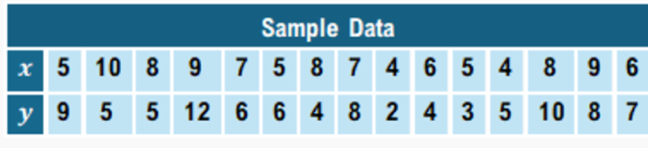
[DATA] Home Runs (Refer to Problem 31, Section 4.1.) The following data represent the speed at which a ball was hit (in miles per hour) and the distance it traveled (in feet) for a random sample of home runs in a Major League baseball game.
b. Explain the meanings of the slope and y-intercept in this context, if appropriate.
27
views

