

 06:46
06:46

Textbook Question
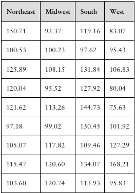
In Exercises 17–20, (a) identify the claim and state H₀ and Hₐ, (b) find the critical value and identify the rejection region, (c) find the test statistic F, (d) decide whether to reject or fail to reject the null hypothesis, and (e) interpret the decision in the context of the original claim. Assume the samples are random and independent, and the populations are normally distributed.
[APPLET] An instructor claims that the variance of SAT evidence-based reading and writing scores is different than the variance of SAT math scores. The table shows the SAT evidence-based reading and writing scores for 12 randomly selected students and the SAT math scores for 12 randomly selected students. At α=0.01, can you support the instructor’s claim?
78
views