Instrument Calibration and Analytical Figures of Merit

Introduction to Calibration in Analytical Chemistry

Calibration is a fundamental process in analytical chemistry that establishes the relationship between the instrument response and the known concentrations of an analyte. This process ensures accurate and reliable quantitative measurements in chemical analysis.

• Calibration Curve: A plot of instrument response (e.g., emission intensity, absorbance) versus analyte concentration. It is used to determine the concentration of unknown samples by interpolation.

• Standard Solutions: Solutions of known concentration used to construct the calibration curve.

• Linearity: The range over which the instrument response is directly proportional to analyte concentration.

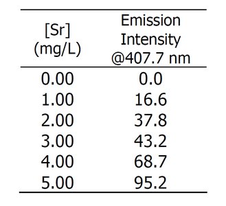
Tabular Data: Calibration Standards

Calibration data are often presented in tables, showing the relationship between analyte concentration and instrument response.

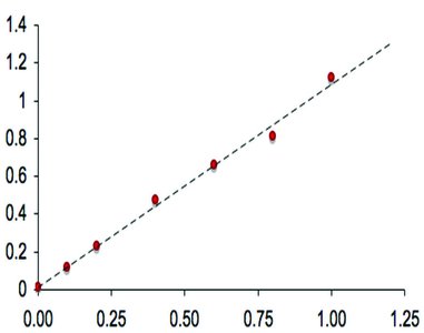
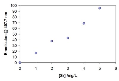
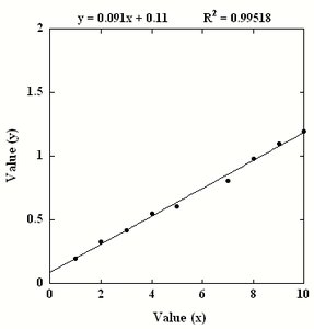
Graphical Representation of Calibration Data

Graphing calibration data helps visualize the relationship and assess linearity, outliers, and the quality of fit.

• Scatter Plot: Plots measured response versus concentration.

• Best-Fit Line: A regression line that best represents the data trend.

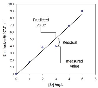
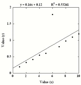
Residuals and Goodness of Fit

Residuals are the differences between measured values and those predicted by the calibration curve. Analyzing residuals helps assess the accuracy of the fit.

• Residual:

• Goodness of Fit (R2): Indicates how well the regression line fits the data. Values close to 1 indicate a good fit.

Analytical Figures of Merit

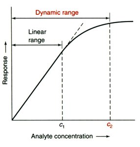
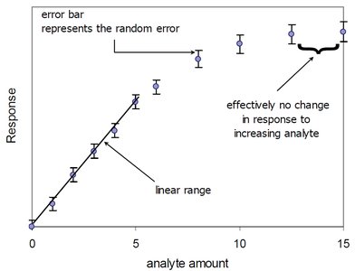
Dynamic Range and Linear Range

The dynamic range of an analytical method is the concentration range over which the instrument provides a measurable response. The linear range is the subset where the response is directly proportional to concentration.

• Dynamic Range: From the lowest detectable concentration (limit of detection) to the highest concentration before response plateaus.

• Linear Range: The range where the calibration curve is a straight line.

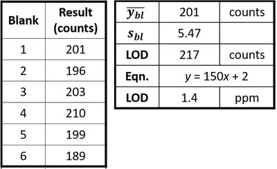
Limit of Detection (LOD) and Limit of Quantitation (LOQ)

The limit of detection (LOD) is the lowest concentration of analyte that can be reliably distinguished from background noise. The limit of quantitation (LOQ) is the lowest concentration that can be quantitatively determined with acceptable precision and accuracy.

• LOD Calculation: , where is the mean blank response and is the standard deviation of the blank.

• LOQ Calculation:

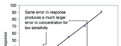
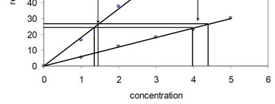
Sensitivity

Sensitivity is the slope of the calibration curve and reflects how much the instrument response changes per unit change in analyte concentration.

• High Sensitivity: Small changes in concentration produce large changes in response.

• Low Sensitivity: Same error in response leads to larger error in calculated concentration.

Statistical Analysis and Error in Calibration

Random and Systematic Errors

Errors in analytical measurements can be classified as random (indeterminate) or systematic (determinate). Random errors cause scatter in data, while systematic errors cause consistent bias.

• Random Error: Reflected in the scatter of points around the calibration line.

• Systematic Error: Causes the calibration line to shift away from the true value.

Outlier Detection and Data Fitting

Outliers can significantly affect the calibration curve and should be identified and addressed. Removing outliers can improve the fit and accuracy of the calibration.

• R2 Value: Indicates the proportion of variance explained by the model. Higher values indicate better fit.

• Data Fitting: Linear regression is commonly used for calibration curves.

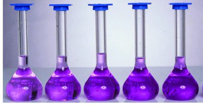
Preparation of Standard Solutions

Serial Dilution and Volumetric Techniques

Accurate preparation of standard solutions is essential for reliable calibration. Serial dilution involves stepwise dilution of a stock solution to prepare a range of concentrations.

• Volumetric Flasks: Used for precise preparation of solutions.

• Serial Dilution: Successive dilutions to achieve desired concentrations.

• Dilution Equation:

Summary Table: Key Analytical Figures of Merit

Conclusion

Understanding calibration, figures of merit, and statistical analysis is essential for accurate quantitative analysis in analytical chemistry. Proper preparation of standards, careful data analysis, and awareness of errors ensure reliable and reproducible results.