Functions and Graphs

Introduction to Functions and Their Graphs

Understanding functions and their graphical representations is foundational in business calculus. A relation is a connection between input (x) and output (y) values, often represented as ordered pairs (x, y). A function is a special type of relation where each input has at most one output.

• Vertical Line Test: A graph represents a function if no vertical line intersects the graph at more than one point.

• Inputs (Domain): The set of all possible x-values.

• Outputs (Range): The set of all possible y-values.

Example: The relation {(−3, 5), (0, 2), (3, 5)} is a function because each input has only one output. The relation {(2, 5), (0, 2), (2, 9)} is not a function because the input 2 has two different outputs (5 and 9).

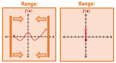
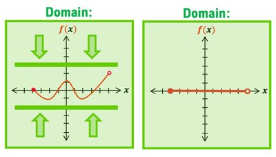
Domain and Range of a Graph

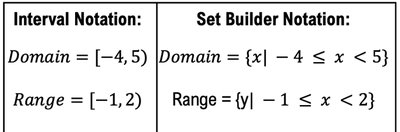
The domain of a graph is the set of allowed x-values, and the range is the set of allowed y-values. To find the domain, project the graph onto the x-axis; for the range, project onto the y-axis. Use interval notation or set builder notation to express these sets.

• Interval Notation: Uses brackets [ ] for inclusion and parentheses ( ) for exclusion.

• Set Builder Notation: Describes the set using inequalities.

• For graphs with multiple intervals, use the union symbol ( ∪ ).

Piecewise Functions

A piecewise function is defined by different equations for different intervals of the domain. If the y-values at the boundaries do not match, the function has a jump, often indicated by open or closed circles on the graph.

• To evaluate a piecewise function at a specific x-value, determine which interval the x-value falls into and use the corresponding equation.

Example: For To find , use ; to find or , use .

Properties of Functions

Functions can be classified and analyzed based on their graphical properties:

• Maximum/Minimum: The highest/lowest point on the graph.

• Increasing/Decreasing: Where the graph rises or falls as x increases.

• Constant: Where the graph is flat (no change in y).

• Symmetry: Even functions are symmetric about the y-axis (); odd functions are symmetric about the origin ().

Graphs of Common Functions

Several basic functions frequently appear in calculus:

• Constant Function:

• Identity Function:

• Square Function:

• Cube Function:

• Square Root Function: (x must be non-negative)

• Cube Root Function: (x can be any real number)

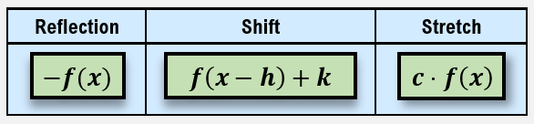
Transformations of Functions

Transformations change the position or shape of a function's graph. The main types are:

• Reflection: Flips the graph over an axis, e.g., .

• Shift: Moves the graph horizontally or vertically, e.g., .

• Stretch/Compression: Multiplies the function by a constant, e.g., .

Operations with Functions

Functions can be added, subtracted, multiplied, or divided. The domain of the resulting function is the intersection of the domains of the original functions (and for division, where the denominator is not zero).

• Addition:

• Subtraction:

• Multiplication:

• Division: ,

Rules of Exponents

Exponent rules are essential for simplifying expressions in calculus:

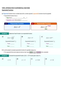
Introduction to Exponential Functions

Exponential functions have the form , where the base is a positive constant not equal to 1. These functions model rapid growth or decay, common in business and economics.

• Domain: All real numbers

• Range: for

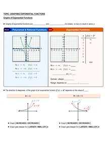
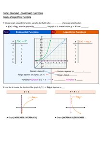
Graphing Exponential Functions

The graph of increases if and decreases if . The y-intercept is always at (0, 1), and the x-axis is a horizontal asymptote.

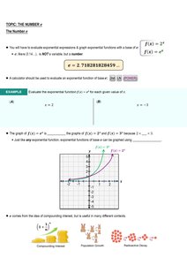
The Number e

The number is a special base for exponential functions, especially in continuous growth and decay models. The function is called the natural exponential function.

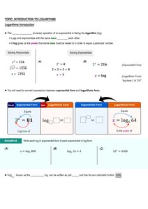
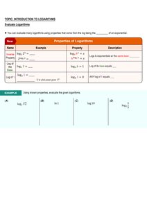
Introduction to Logarithms

A logarithm is the inverse of an exponential function. If , then . Logarithms are used to solve equations involving exponents.

• Common Logarithm: Base 10, written as

• Natural Logarithm: Base , written as

Graphing Logarithmic Functions

The graph of is the inverse of . The domain is , and the range is all real numbers. The y-axis is a vertical asymptote.

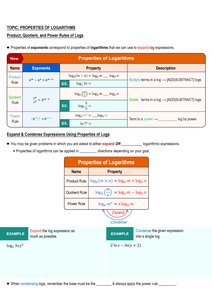
Properties of Logarithms

Logarithms have several important properties for simplifying expressions:

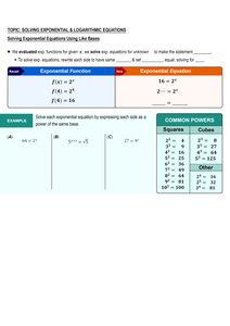
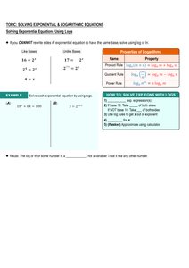
Solving Exponential and Logarithmic Equations

To solve exponential equations, express both sides with the same base if possible, or use logarithms. To solve logarithmic equations, use properties of logarithms to combine or expand expressions, then rewrite in exponential form if needed.

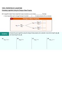
Change of Base Property

The change of base formula allows you to evaluate logarithms with any base using common or natural logarithms:

• , where is any positive value (commonly 10 or ).

Summary Table: Function Transformations

Additional info: These foundational concepts are essential for understanding calculus topics such as limits, derivatives, and integrals, especially in business applications involving growth, decay, and optimization.