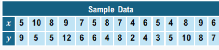
Using the sample data below, run a hypothesis test on $β$ to see if there is evidence that there is a positive correlation between $x$ and $y$ with $alpha equals 0.01$ .

Reject $H_0$ and conclude that there is a positive correlation between $x$ and $y$ and that $\beta>0$ .

Fail to reject $H_0$ since there is enough evidence to suggest $\beta>0$ , but not enough evidence to suggest positive linear correlation between $x$ and $y$ .

Fail to reject $H_0$ since there is not enough evidence to suggest $\beta>0$ and not enough evidence to suggest positive linear correlation between $x$ and $y$ .

Reject $H_0$ since there is not enough evidence to suggest $\beta>0$ and not enough evidence to suggest positive linear correlation between $x$ and $y$ .

Verified step by step guidance

Step 1: Define the hypotheses for the test. The null hypothesis ($H_0$) states that there is no positive correlation between $x$ and $y$, which means $\beta \leq 0$. The alternative hypothesis ($H_a$) states that there is a positive correlation, so $\beta > 0$.

Step 2: Calculate the sample correlation coefficient $r$ between the paired $x$ and $y$ values using the formula: \[r = \frac{n\sum xy - \sum x \sum y}{\sqrt{(n\sum x^2 - (\sum x)^2)(n\sum y^2 - (\sum y)^2)}}\] where $n$ is the number of pairs.

Step 3: Compute the test statistic $t$ for the correlation using the formula: \[t = \frac{r\sqrt{n-2}}{\sqrt{1-r^2}}\] This follows a $t$-distribution with $n-2$ degrees of freedom.

Step 4: Determine the critical value from the $t$-distribution for a one-tailed test at the significance level $\alpha = 0.01$ with $n-2$ degrees of freedom.

Step 5: Compare the calculated test statistic $t$ to the critical value. If $t$ is greater than the critical value, reject $H_0$ and conclude there is evidence of a positive correlation. Otherwise, fail to reject $H_0$, indicating insufficient evidence to support a positive correlation between $x$ and $y$.

4:30m

Watch next

Master Hypothesis Test for the Slope of a Regression Line with a bite sized video explanation from Patrick

Inferences for Slope practice set

Problem sets built by lead tutors

Expert video explanations

Struggling with Statistics for Business?

Using the sample data below, run a hypothesis test on ββ to see if there is evidence that there is a positive correlation between xx and yy with α=0.01\alpha=0.01.

Watch next

Inferences for Slope practice set

Using the sample data below, run a hypothesis test on $β$ to see if there is evidence that there is a positive correlation between $x$ and $y$ with $alpha equals 0.01$ .