Chapter 3: Probability

3.1 Events, Sample Spaces, and Probability

Probability theory forms the foundation for statistical inference and decision-making in business. Understanding the basic concepts of experiments, sample spaces, and events is essential for analyzing uncertainty.

• Experiment: A process of observation that leads to a single outcome, which cannot be predicted with certainty.

• Sample Point: The most basic outcome of an experiment.

• Sample Space (S): The collection of all possible sample points. Written as S = {list of sample points}.

• Event: A specific collection of sample points. Events can be simple (one sample point) or compound (two or more sample points).

• Probability: The likelihood of occurrence of an event, assigned to each sample point.

Example: Flipping a coin once yields sample points: Heads (H) or Tails (T). The sample space is S = {H, T}.

Example: Flipping two coins yields sample points: HH, HT, TH, TT. The sample space is S = {HH, HT, TH, TT}.

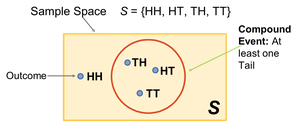
Events Visualized: For the experiment of flipping two coins, the event 'at least one tail' includes sample points HT, TH, TT.

Steps for Calculating Probability of Events:

1. Define the experiment and describe the observation process.

2. List the sample points.

3. Assign probabilities to the sample points.

4. Determine the collection of sample points in the event of interest.

5. Sum the probabilities of the sample points to get the event probability.

Example: Two smartphones are randomly selected from an assembly line. The sample points and their probabilities are:

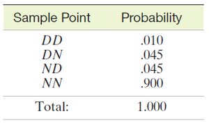
Example: Event A = {Observe exactly one defective: DN, ND}, Event B = {Observe at least one defective: DN, ND, DD}. Probability of A = P(DN) + P(ND) = 0.045 + 0.045 = 0.090. Probability of B = P(DN) + P(ND) + P(DD) = 0.045 + 0.045 + 0.010 = 0.100.

Combinations Rule

Combinatorial rules help determine the number of possible outcomes in experiments involving selection or arrangement.

• Example: Forming pairs from four students (Amy, John, Bob, Sue) yields six possible pairs: Amy-John, Amy-Bob, Amy-Sue, John-Bob, John-Sue, Bob-Sue.

• Example: Selecting five ventures from twenty: The number of samples is given by the combination formula , where n = 20, r = 5.

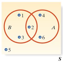
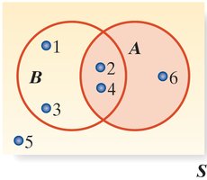
3.2 Union and Intersection

Unions and intersections are fundamental operations for combining events in probability theory. Venn diagrams are used to visualize these relationships.

• Union (A ∪ B): The event that either A or B or both occur. The union includes all sample points in A, B, or both.

• Intersection (A ∩ B): The event that both A and B occur. The intersection includes only sample points common to both A and B.

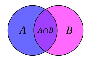
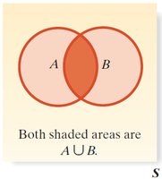
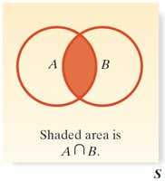
Example: If A = {4, 6}, B = {1, 2, 3}, then A ∪ B = {1, 2, 3, 4, 6}, A ∩ B = {2}.

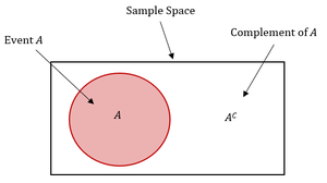
3.3 Complementary Events

The complement of an event consists of all sample points in the sample space that are not in the event. The probability of the complement is one minus the probability of the event.

• Complementary Event (Ac): All outcomes not in event A.

• Rule of Complements:

Example: If 37 out of 50 customers live within 3 miles of a store, the probability that a randomly selected customer lives within 3 miles is . The probability that a customer does not live within 3 miles is .

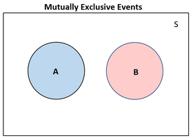
3.4 The Additive Rule and Mutually Exclusive Events

The additive rule is used to calculate the probability of the union of two events. If events are mutually exclusive, their intersection is empty.

• Additive Rule:

• Mutually Exclusive Events: Events that cannot occur together; .

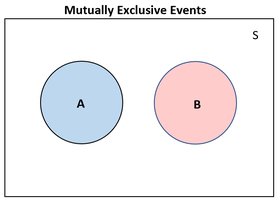
Example: If A and B are mutually exclusive, .

3.5 Conditional Probability

Conditional probability measures the likelihood of an event given that another event has occurred. It is a key concept in risk assessment and business decision-making.

• Conditional Probability:

Example: In a study, 55% of executives cheated at golf, and 20% cheated at golf and lied in business. The probability that an executive lied in business given they cheated at golf is:

3.6 The Multiplicative Rule and Independent Events

The multiplicative rule is used to find the probability of the intersection of two events. If events are independent, the occurrence of one does not affect the probability of the other.

• Multiplicative Rule:

• Independent Events:

Example: Tossing a fair die: A = {even number}, B = {number ≤ 4}. To check independence, compare to .

Example: An investor estimates the probability of profitable wheat production given a drought is 0.01, and the probability of a drought is 0.05. The probability of both events is .

Summary Table: Probability Concepts