Introduction to Hypothesis Testing

Overview of Hypothesis Testing

Hypothesis testing is a fundamental statistical method used to make inferences about population parameters based on sample data. It involves formulating a statement (hypothesis) about a population parameter and using sample evidence to determine whether to reject or fail to reject that statement.

• Null Hypothesis (H0): The default assumption or status quo about a population parameter, assumed true unless strong evidence suggests otherwise.

• Alternative Hypothesis (HA or H1): The competing claim, considered true if the null hypothesis is rejected.

• Decision: Based on sample data, we either reject H0 or do not reject H0.

Examples of Hypothesis Testing in Practice

• Drug Safety: The FDA requires sufficient evidence before certifying a drug as safe and effective.

• Manufacturing: Testing if orange juice bottles are filled to the correct amount (e.g., 32 ounces).

• Legal System: Presumption of innocence is the null hypothesis; evidence must be strong to reject it.

Formulating Hypotheses

Steps in Formulating Hypotheses

Formulating hypotheses involves identifying the population parameter, stating the null and alternative hypotheses, and determining the direction of the test.

• Step 1: Identify the population parameter (e.g., mean μ, proportion p).

• Step 2: State the null hypothesis (H0) with equality (e.g., μ ≤ 20).

• Step 3: State the alternative hypothesis (HA) reflecting the claim or research question (e.g., μ > 20).

One-Tailed vs. Two-Tailed Tests

• One-Tailed Test: The rejection region is in one tail of the distribution (e.g., testing if μ > μ0).

• Two-Tailed Test: The rejection region is split between both tails (e.g., testing if μ ≠ μ0).

Types of Statistical Errors

Type I and Type II Errors

Statistical errors occur when the sample leads to an incorrect conclusion about the population.

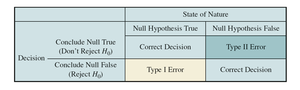
• Type I Error (α): Rejecting H0 when it is actually true (false alarm).

• Type II Error (β): Failing to reject H0 when it is actually false (missed detection).

Significance Level and Critical Value

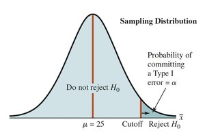
Significance Level (α)

The significance level is the maximum probability of committing a Type I error that the researcher is willing to accept. Common values are 0.05 or 0.01.

Critical Value

The critical value is the threshold that determines the boundary of the rejection region for the test statistic. If the test statistic exceeds the critical value, the null hypothesis is rejected.

• zα: The critical z-value from the standard normal distribution.

Test Statistics and Decision Rules

z-Test Statistic for Means (σ Known)

When the population standard deviation (σ) is known, the z-test statistic is used:

• \( \bar{x} \): Sample mean

• \( \mu \): Hypothesized population mean

• \( \sigma \): Population standard deviation

• \( n \): Sample size

Decision Rule Example

For a right-tailed test, reject H0 if the test statistic is greater than the critical value.

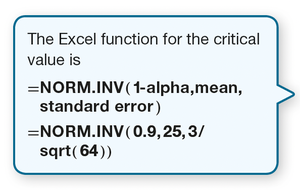
Using Excel for Critical Values

Excel can be used to compute the critical value for a given significance level:

• =NORM.INV(1-alpha, mean, standard error)

• Example: =NORM.INV(0.9, 25, 3/sqrt(64))

p-Value Approach

Definition and Use

The p-value is the probability, assuming the null hypothesis is true, of obtaining a test statistic as extreme as the observed value. If the p-value is less than the significance level (α), reject H0.

• p-value < α: Reject H0

• p-value ≥ α: Do not reject H0

t-Test Statistic for Means (σ Unknown)

t-Test Statistic

When the population standard deviation is unknown and the sample size is small, the t-test statistic is used:

• \( s \): Sample standard deviation

• Other symbols as above

Hypothesis Tests for Proportions

z-Test Statistic for Proportions

For large samples, the sampling distribution of the sample proportion is approximately normal. The z-test statistic for proportions is:

• \( \hat{p} \): Sample proportion

• \( p \): Hypothesized population proportion

• \( n \): Sample size

Requirements: Both np ≥ 5 and n(1-p) ≥ 5.

Worked Examples

Example: One-Tailed Hypothesis Test for Mean (σ Known)

• Claim: Mean service time is ≤ 40 minutes (H0: μ ≤ 40, HA: μ > 40)

• Sample: n = 100, σ = 8, sample mean = 43.5, α = 0.05

• Critical z-value: 1.645

• Test statistic:

• Decision: 4.375 > 1.645, so reject H0

• Conclusion: Sufficient evidence that mean service time exceeds 40 minutes.

Example: Hypothesis Test for a Proportion

• Claim: Proportion of cancellations ≤ 10% (H0: p ≤ 0.10, HA: p > 0.10)

• Sample: n = 100, sample proportion = 0.14, α = 0.05

• Test statistic:

• Decision: 1.33 < 1.645, so do not reject H0

• Conclusion: Insufficient evidence that more than 10% will cancel.

Summary Table: Hypothesis Testing Steps