Chapter 10 & 11: Sampling Distributions and Confidence Intervals for Proportions

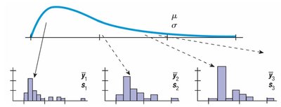
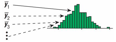
Sampling Distributions and the Central Limit Theorem (CLT)

The Central Limit Theorem (CLT) is a foundational concept in statistics, stating that the sampling distribution of the sample mean (or proportion) will be approximately Normal, regardless of the population's distribution, provided the sample size is sufficiently large. This allows statisticians to make inferences about population parameters using sample statistics.

• Sampling Distribution: The probability distribution of a statistic (such as the mean or proportion) calculated from multiple samples drawn from the same population.

• Sample Mean: An unbiased estimate of the population mean.

• Standard Error: Measures the variability of the sample statistic. For the mean: (or if is unknown).

• Cases for Sampling Distribution: Depending on population shape, known/unknown standard deviation, and sample size, different distributions and test statistics are used (Normal or t-distribution).

Sampling Distribution of Sample Proportion

The sample proportion () is an unbiased estimate of the population proportion (). For large samples, the sampling distribution of $\hat{p}$ is approximately Normal.

• Shape: Normal if sample size is large and is not near 0 or 1.

• Mean:

• Standard Error:

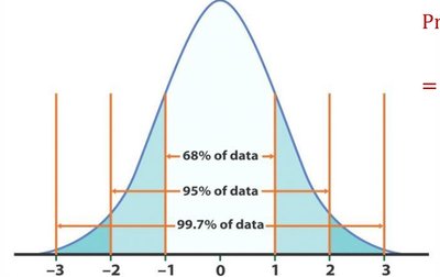
Recap of the Normal Distribution

The Normal (Gaussian) distribution is the most commonly used distribution in statistics, characterized by its mean () and standard deviation (). It is symmetric and used to model many real-world phenomena.

• Standard Normal Distribution: , mean 0, SD 1.

• Empirical Rule: 68% of data within ±1 SD, 95% within ±2 SD, 99.7% within ±3 SD.

Standardization and z-distribution

Any Normal random variable can be standardized to the z-distribution using . This allows calculation of probabilities and critical values for hypothesis testing and confidence intervals.

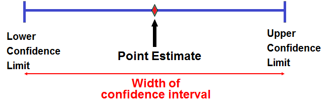
Confidence Intervals for Proportions

A confidence interval provides a range of values within which the true population proportion is likely to fall, based on the sample proportion and the margin of error.

• Generic Formula: Point Estimate ± Margin of Error

• Margin of Error:

• Standard Error:

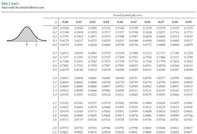
• Critical Value: from the Standard Normal table, depending on confidence level.

Interpretation of Confidence Intervals

Confidence intervals are interpreted as follows:

• "We are 95% confident that the true proportion lies between the lower and upper bounds."

• In repeated sampling, 95% of constructed intervals will contain the true proportion.

• Uncertainty is about whether the particular sample interval contains the true value.

Margin of Error: Certainty vs Precision

The margin of error reflects the uncertainty in the estimate. Higher confidence levels increase the margin of error, making the interval wider but less precise. Lower confidence levels decrease the margin of error, making the interval narrower but less certain.

• Trade-off: Certainty vs Precision. 100% confidence yields a very wide interval; lower confidence yields a narrower, more precise interval.

Critical Values and Standard Normal Tables

Critical values () are determined from the Standard Normal distribution and depend on the desired confidence level.

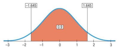
• 90% confidence:

• 95% confidence:

• 99% confidence:

Assumptions and Conditions for Confidence Intervals

Before constructing a confidence interval, check these conditions:

• Independence: Data values must not affect each other.

• Randomization: Data must be randomly sampled.

• 10% Condition: Sample size should be no more than 10% of the population if sampling without replacement.

• Success/Failure Condition: Both and .

Example: Confidence Interval for Proportion

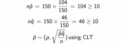
Suppose 104 out of 150 college students played soccer in their youth. Estimate the proportion with a 98% confidence interval.

• Check conditions: ,

• Calculate

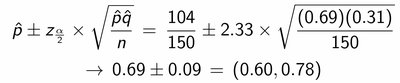
• Critical value for 98%:

• Confidence interval:

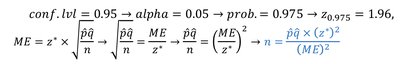
Choosing the Sample Size

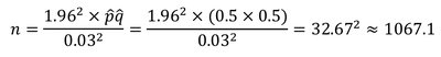
To estimate a proportion with a desired margin of error and confidence level, solve for sample size :

• If no prior estimate for , use (worst case scenario).

• Always round up the calculated .

Summary Table: Common Confidence Levels and Critical Values

Key Formulas

• Confidence Interval for Proportion:

• Sample Size: