Describing Data Using Numerical Measures

Overview

This chapter introduces key numerical measures used to describe and analyze data in business statistics. These measures help summarize data sets, identify central tendencies, and assess variability, providing a foundation for statistical decision-making.

Measures of Center and Location

Parameters vs. Statistics

Measures of center and location are used to summarize the central value of a data set. A parameter is a measure computed from the entire population, typically denoted by Greek letters. A statistic is a measure computed from a sample, denoted by Roman letters.

Population Mean

The mean (average) is a fundamental measure of center. For a population, it is calculated as:

• Formula:

• Where: = population mean, = population size, = ith value

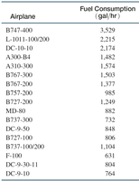
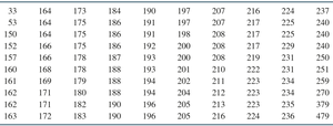
Example: The mean fuel consumption rate for 17 airplanes is calculated by summing all hourly rates and dividing by 17.

Sample Mean

For a sample, the mean is:

• Formula:

• Where: = sample mean, = sample size, = ith value

Example: The mean salary for a sample of seven data analysts is calculated by summing their salaries and dividing by 7.

Impact of Extreme Values

The mean is sensitive to extreme values (outliers), which can skew the measure of center. In such cases, the median may be more appropriate.

Median

The median is the middle value when data are sorted. It divides the data into two equal halves.

• Arrange data in order.

• Median index:

• If is not an integer, round up; if is an integer, average the values at positions and .

Example: For seven sorted salaries, the median is the fourth value.

Skewed and Symmetric Distributions

Data distributions can be symmetric or skewed. The relationship between mean and median indicates skewness:

• Symmetric: Mean = Median

• Right-skewed: Mean > Median

• Left-skewed: Mean < Median

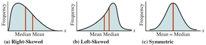
Advantage: The median is not affected by extreme values.

Mode

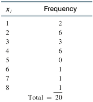
The mode is the value that occurs most frequently in a data set. A set may have more than one mode or none.

• Mode is not always near the center.

• Example: Group sizes in a restaurant, where modes are 2 and 4.

Other Measures of Location

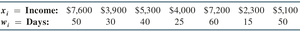
• Weighted Mean: Accounts for varying importance of data values.

• Percentiles: The pth percentile divides data so that at least p% are below and (100-p)% are above.

• Quartiles: Divide data into four equal parts; Q1 (25th percentile), Q2 (median), Q3 (75th percentile).

Percentiles and Quartiles

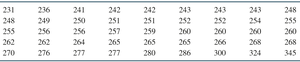
Percentiles and quartiles are calculated by sorting data and finding the location index:

• Percentile Location Index:

• Round up if not integer; average values if integer.

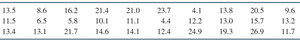
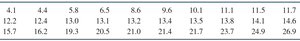
Example: The 80th percentile is the average of the 24th and 25th values.

Box and Whisker Plots

Box and Whisker Plot Construction

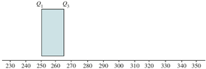
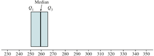
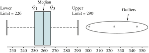
A box and whisker plot visually displays the five-number summary: minimum, Q1, median, Q3, and maximum. It helps identify outliers.

• Box spans Q1 to Q3; median marked inside box.

• Whiskers extend to values within 1.5 IQR of Q1 and Q3.

• Outliers are marked outside whiskers.

Measures of Variation

Range

The range is the difference between the maximum and minimum values:

• Formula:

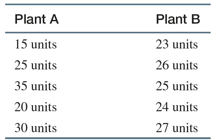
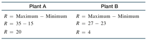
Limitation: Range is sensitive to extreme values and only uses two data points.

Interquartile Range (IQR)

The interquartile range measures spread using quartiles:

• Formula:

• Less sensitive to extreme values than range.

Example: IQR is calculated as the difference between the 75th and 25th percentiles.

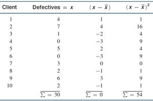
Variance and Standard Deviation

Variance measures the average squared deviation from the mean. Standard deviation is the square root of variance and has the same units as the original data.

• Population Variance:

• Population Standard Deviation:

• Sample Variance:

• Sample Standard Deviation:

Using the Mean and Standard Deviation Together

Coefficient of Variation (CV)

The coefficient of variation expresses standard deviation as a percentage of the mean, allowing comparison of variability across different data sets.

• Population CV:

• Sample CV:

The Empirical Rule

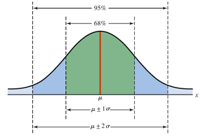
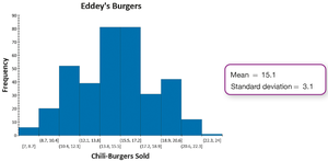
Empirical Rule for Bell-Shaped Distributions

If data are approximately normal (bell-shaped):

• 68% of values fall within 1 standard deviation of the mean

• 95% within 2 standard deviations

• Almost all within 3 standard deviations

Tchebysheff’s Theorem

Tchebysheff’s theorem applies to any data distribution, stating that at least of values fall within standard deviations of the mean, for .

• For , at least 75% of values

• For , at least 89% of values

Standardized Data Values (z-scores)

Definition and Calculation

A z-score indicates how many standard deviations a value is from the mean.

• Population z-score:

• Sample z-score:

Application: Standardized scores allow comparison across different distributions, such as SAT and ACT scores.

Additional info: All examples, tables, and images are directly relevant to the explanation of the corresponding statistical concepts and their business applications.