Estimating Single Population Parameters

Point and Confidence Interval Estimates for a Population Mean

Estimating population parameters is a fundamental task in business statistics. This section introduces the concepts of point estimates and confidence intervals, which are used to infer population characteristics from sample data.

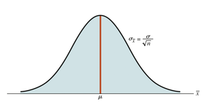
• Point Estimate: A single statistic calculated from a sample, used to estimate the corresponding population parameter. For example, the sample mean (\bar{x}) is a point estimate of the population mean (\mu).

• Sampling Error: The difference between a sample statistic and the actual population parameter. Sampling error arises because only a subset of the population is observed.

• Example: If a poll finds that 82% of sampled adults favor banning texting while driving, 82% is the point estimate for the population proportion.

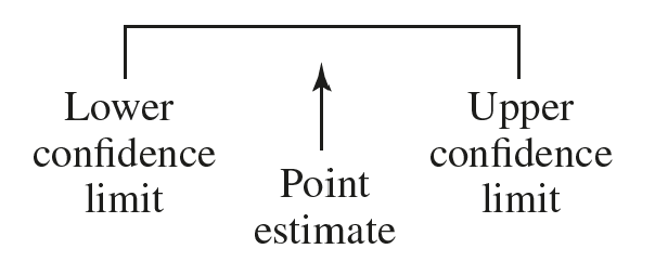
Confidence Intervals

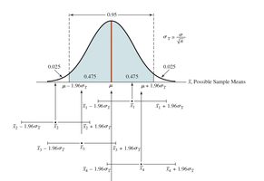
A confidence interval provides a range of values, derived from sample data, that is likely to contain the population parameter. The confidence level (e.g., 95%) indicates the proportion of such intervals that would contain the parameter if repeated samples were taken.

• Confidence Interval: An interval constructed from sample values, such that a specified percentage of all possible intervals will include the true population parameter.

• Interpretation: If all possible intervals were constructed from a given sample size, 95% would include the population mean (\mu).

Business Application: Health Star Energy Drink Example

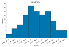
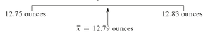
Consider a company that fills energy drink bottles. The fill machine has a known standard deviation (\sigma = 0.2 ounces). A sample of 100 bottles yields a sample mean of 12.79 ounces. The manager wants to estimate the mean fill for all bottles.

• Sample Mean: \bar{x} = 12.79 ounces

• Population Standard Deviation: \sigma = 0.2 ounces

• Sample Size: n = 100

• 95% Confidence Interval: 12.75 ounces to 12.83 ounces

• Interpretation: Since the interval does not contain the target mean of 12 ounces, the machine is overfilling.

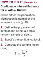
Constructing a Confidence Interval Estimate for μ (σ Known)

When the population standard deviation is known, the confidence interval for the mean is calculated using the z-distribution.

1. Define the population and select a random sample of size n.

2. Specify the confidence level (e.g., 95%).

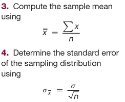
3. Compute the sample mean:

4. Determine the standard error:

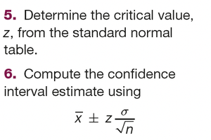
5. Find the critical value z for the desired confidence level.

6. Compute the confidence interval:

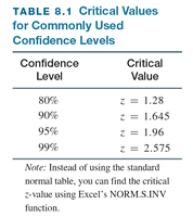
Critical Values for Common Confidence Levels

The critical value z depends on the confidence level. Common values are:

Margin of Error

The margin of error is the amount added to and subtracted from the point estimate to determine the endpoints of the confidence interval. It quantifies the expected closeness of the estimate to the population parameter.

• Formula:

• Impact of Confidence Level: Higher confidence levels increase the margin of error; lower levels decrease it.

• Impact of Sample Size: Increasing sample size reduces the margin of error.

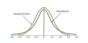
Student’s t-Distributions (σ Unknown)

When the population standard deviation is unknown, the t-distribution is used. The t-distribution is bell-shaped and symmetric, but has heavier tails than the normal distribution. It is defined by degrees of freedom (df = n - 1).

• Formula for Confidence Interval:

• Degrees of Freedom: Number of independent values used to estimate the population standard deviation.

• As sample size increases: The t-distribution approaches the normal distribution.

Business Application: Eastern Automotive Protection Example

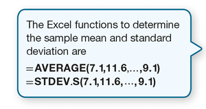
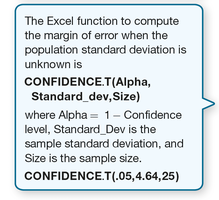
A team samples 25 customer calls to estimate the mean call time. The sample mean is 7.088 minutes, sample standard deviation is 4.64 minutes, and the 95% confidence interval is calculated using the t-distribution.

• Sample Mean: 7.088 minutes

• Sample Standard Deviation: 4.64 minutes

• Sample Size: 25

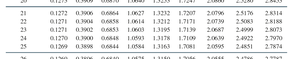
• Degrees of Freedom: 24

• Critical t-value: 2.0639

• 95% Confidence Interval: 5.173 minutes to 9.003 minutes

Determining Required Sample Size for Estimating a Population Mean

Business decision makers often need to know how large a sample is required to achieve a desired margin of error at a specified confidence level.

• Sample Size Formula (σ Known):

• Sample Size Formula (σ Unknown): Use sample standard deviation from a pilot sample.

• Example: For a margin of error of 0.50 gallons, σ = 4.85, z = 1.645 (90% confidence), required sample size is 255.

Estimating a Population Proportion

Population proportion (p) is estimated using the sample proportion (\hat{p}). Confidence intervals for proportions are constructed similarly to those for means.

• Sample Proportion: , where x is the number of items with the attribute of interest.

• Standard Error:

• Confidence Interval:

• Example: In a sample of 100 customers, 62 use a voucher. The 95% confidence interval for the proportion is 52.5% to 71.5%.

Summary Table: Key Formulas

Additional info:

• Increasing sample size or lowering population standard deviation reduces margin of error.

• Confidence intervals are not probability statements about the parameter, but about the method.

• The t-distribution is used when σ is unknown and n is small.