Introduction to Continuous Probability Distributions

This chapter introduces the foundational concepts of continuous probability distributions, focusing on the normal, uniform, and exponential distributions. These distributions are essential for modeling and analyzing real-world business data where outcomes are measured on a continuous scale.

Section 6.1: The Normal Probability Distribution

Definition and Properties

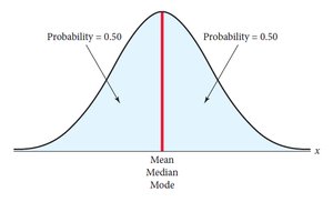
The normal probability distribution is a continuous, bell-shaped distribution that is widely used in statistics due to its natural occurrence in many real-world phenomena.

• Unimodal: The distribution has a single peak.

• Symmetrical: The left and right sides of the distribution are mirror images.

• Mean, Median, and Mode: All are equal and located at the center of the distribution.

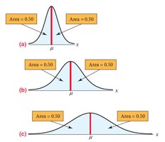
Normal Distribution Variations

Different normal distributions can be generated by changing the mean (μ) and standard deviation (σ):

• Changing μ shifts the distribution left or right.

• Changing σ increases or decreases the spread (width) of the distribution.

Normal Probability Density Function

The probability density function (PDF) for a normal distribution is:

• x: Value of the continuous random variable

• μ: Population mean

• σ: Population standard deviation

• e: Base of the natural logarithm (≈ 2.71828)

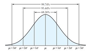
Empirical Rule (68-95-99.7 Rule)

The empirical rule describes the approximate percentage of data within certain standard deviations from the mean:

• 68.26% within ±1σ

• 95.44% within ±2σ

• 99.74% within ±3σ

Finding Normal Probabilities

For a continuous random variable, the probability that it falls within a range is the area under the curve between two values:

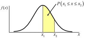
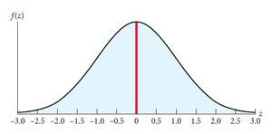
The Standard Normal Distribution

The standard normal distribution is a special case of the normal distribution with mean 0 and standard deviation 1. The horizontal axis is scaled in z-values, which measure the number of standard deviations a point is from the mean.

• Values above the mean have positive z-values.

• Values below the mean have negative z-values.

Standardizing a Normal Variable

Any normal distribution can be converted to the standard normal distribution using the z-score formula:

• z: Standardized value

• x: Value from the original distribution

• μ: Mean of the original distribution

• σ: Standard deviation of the original distribution

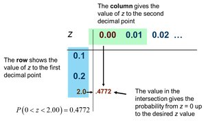
Using the Standard Normal Table

The standard normal table (z-table) provides the area (probability) to the left of a given z-value. To find probabilities for a range, subtract the areas as needed.

Examples of Normal Probability Calculations

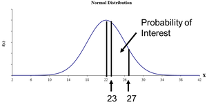
Gas Mileage Example

Suppose gas mileage for a new SUV is normally distributed with μ = 22 mpg and σ = 4 mpg. Find the probability that a randomly selected SUV gets between 23 and 27 mpg.

• Convert x-values to z-scores.

• Use the z-table to find the area between the two z-values.

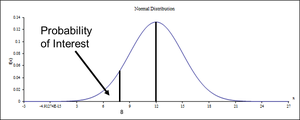
Restaurant Tip Example

Tips left by customers are normally distributed with mean $12.00 and standard deviation $3.00. What is the probability a tip is less than $8.00?

• Convert $8.00 to a z-score.

• Find the corresponding probability using the z-table.

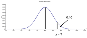
Entrance Exam Score Example

Entrance exam scores are normally distributed with mean 800 and standard deviation 50. To admit the top 10% of students, what should the cutoff score be?

• Find the z-value corresponding to the top 10% (z ≈ 1.28).

• Solve for x using the z-score formula.

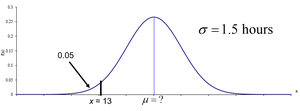
Cell Phone Battery Example

Battery life is normally distributed with σ = 1.5 hours. To ensure no more than 5% of batteries last 13 hours or less, what must the mean be?

• Find the z-value for the lower 5% (z ≈ -1.645).

• Solve for μ using the z-score formula.

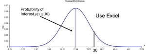
Job Completion Times Example

Production time for patio sets is normally distributed with mean 22.14 minutes and σ = 6.09 minutes. What proportion are completed in 30 minutes or less?

• Convert 30 minutes to a z-score.

• Find the cumulative probability using the z-table or Excel.

Excel Applications

Excel functions such as NORM.DIST and EXPON.DIST can be used to compute probabilities for normal and exponential distributions, respectively.

Section 6.2: Other Continuous Probability Distributions

Uniform Probability Distribution

The uniform distribution is a continuous probability distribution where all intervals of the same length within the range are equally probable. The PDF is constant between the minimum (a) and maximum (b) values.

• a: Minimum value

• b: Maximum value

The graph of the uniform distribution is a rectangle.

Mean and Standard Deviation of Uniform Distribution

Service Time Example

If the time for a dentist examination is uniformly distributed between 15 and 20 minutes, the probability of an exam taking 17 or fewer minutes is:

• Calculate the proportion of the interval [15, 17] within [15, 20].

The Exponential Probability Distribution

The exponential distribution models the time between events in a Poisson process (e.g., time between arrivals or failures). The PDF is:

• μ: Mean time between events

Exponential Probability Calculation

The probability that the time between events exceeds a value a is:

911 Calls Example

If the mean time between 911 calls is 8 minutes, the probability that the time between two calls exceeds 14 minutes is:

• Use the formula

Excel Application for Exponential Distribution

Use EXPON.DIST in Excel to compute probabilities for exponential distributions by supplying x and λ (where λ = 1/μ).

Additional info: This summary expands on the provided slides by including explicit formulas, definitions, and step-by-step explanations for each distribution and example, ensuring the notes are self-contained and suitable for exam preparation.