Random Variables and Probability Distributions

Introduction

Random variables are fundamental to probability and statistics, representing numerical outcomes of random experiments. This chapter explores the types of random variables, their probability distributions, and key models such as the binomial and normal distributions.

Types of Random Variables

Discrete vs. Continuous Random Variables

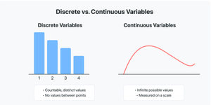
Random variables are classified as either discrete or continuous, depending on the nature of their possible values.

• Discrete Random Variable: Assumes a countable number of values, such as integers or finite sets.

• Continuous Random Variable: Assumes an infinite number of values within an interval, typically measured on a scale.

Examples:

• Discrete: Number of sales, number of customers, number of errors.

• Continuous: Weight of steak, time to complete a task.

Probability Distributions for Discrete Random Variables

Discrete Probability Distribution

A discrete probability distribution assigns probabilities to each possible value of a discrete random variable. This can be represented as a graph, table, or formula.

• Probability Mass Function (PMF): The function that gives the probability for each value.

• Conditions: The sum of all probabilities must equal 1, and each probability must be between 0 and 1.

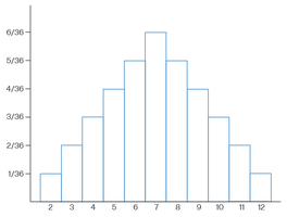
Table Example

Probability distributions can be constructed from frequency tables.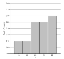

Example: Insurance Application

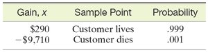
Suppose an insurance company sells a $10,000 policy at an annual premium of $290. The probability of death during the year is 0.001. The expected gain for the company is calculated using the probability distribution:

The Binomial Distribution

Definition and Characteristics

The binomial distribution models the number of successes in a fixed number of independent trials, each with two possible outcomes (success or failure).

• Characteristics:

  • n identical trials

  • Two outcomes per trial (S for success, F for failure)

  • Probability of success (p) is constant; probability of failure (q = 1 - p)

  • Trials are independent

  • Random variable x counts the number of successes

Binomial Probability Formula

The probability of observing x successes in n trials is given by: Example: If a machine produces 10% defectives, and 5 items are tested, the probability that 3 are defective is calculated using the binomial formula.

Probability Distributions for Continuous Random Variables

Continuous Probability Density Function (PDF)

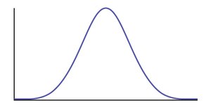
For continuous random variables, the probability distribution is represented by a smooth curve called the probability density function (PDF).

• Key Point: The area under the curve between two points represents the probability that the variable falls within that interval.

The Normal Distribution

Definition and Properties

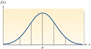
The normal distribution is a continuous probability distribution that is symmetric and bell-shaped.

• Mean, median, and mode are equal.

• Empirical Rule: Approximately 68% of values fall within one standard deviation of the mean, 95% within two, and 99.7% within three.

Effect of Mean and Standard Deviation

Different normal distributions are distinguished by their mean (μ) and standard deviation (σ).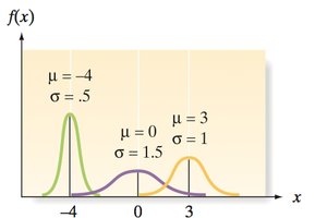

Standard Normal Distribution

The standard normal distribution has a mean of 0 and a standard deviation of 1. Probabilities are found using the z-table.

Finding Probabilities Using the z-table

• Sketch the distribution and shade the area of interest.

• Use the z-table to find the area corresponding to the z-value.

• Apply symmetry as needed.

Example: Cell Phone Application

If the length of time between charges is normally distributed with mean 10 hours and standard deviation 1.5 hours, the probability that the phone lasts between 8 and 12 hours is found by converting to z-scores and using the z-table.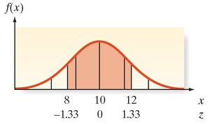

Example: Advertised Gas Mileage

For a car with mean mileage 27 mpg and standard deviation 3 mpg, the probability that a car gets less than 20 mpg is found by calculating the z-score for 20 and finding the corresponding area.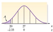

Summary Table: Discrete vs. Continuous Variables

Key Formulas

Mean of Discrete Random Variable

Variance of Discrete Random Variable

Binomial Probability

Standard Normal z-score

Conclusion

Understanding random variables and their probability distributions is essential for analyzing data and making statistical inferences. The binomial and normal distributions are particularly important models in business statistics, providing tools for probability calculations and decision-making.