Simple Linear Regression Analysis

Introduction to Regression Analysis

Regression analysis is a statistical method used to examine the relationship between a quantitative response variable and one or more explanatory quantitative variables. In simple linear regression, we focus on the relationship between two variables: one independent (explanatory) variable and one dependent (response) variable. The primary goal is to predict the value of the response variable based on the value of the explanatory variable.

• Explanatory variable (X): The variable used to explain or predict changes in the response variable (e.g., price).

• Response variable (Y): The variable being predicted or explained (e.g., sales in number of packs).

Example: Jenny wants to study the relationship between the sale price and the number of 12-packs sold of a particular brand of beer. She collects data from 52 stores.

Scatterplot and Regression Line

The relationship between the two variables is first visualized using a scatterplot, where each point represents an observation (a pair of X and Y values). The regression line, also known as the best fit line or Ordinary Least Squares (OLS) Regression Line, is fitted to the data to model this relationship.

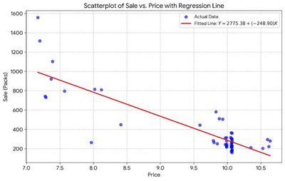
The regression equation from the sample is:

• Interpretation: For each $1 increase in price, the predicted number of packs sold decreases by about 249.

Key Components of Simple Linear Regression

Regression Equation and Parameters

The general form of the sample regression equation is:

• : Predicted value of the response variable for a given x.

• (Sample y-intercept): Predicted mean value of y when x = 0 (may not always be meaningful in context).

• (Sample slope): Predicted change in y for each one-unit increase in x.

Correlation Coefficient (r)

The correlation coefficient (r) measures the strength and direction of the linear relationship between X and Y. Its value ranges from -1 to 1.

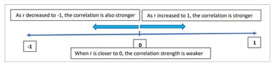
• r close to 1: Strong positive linear relationship.

• r close to -1: Strong negative linear relationship.

• r close to 0: Weak or no linear relationship.

Coefficient of Determination (R2)

R2 measures the proportion of the observed variation in y that can be explained by x. It ranges from 0 to 1.

• High R2: Model explains a large proportion of the variance in the response variable.

• Low R2: Model explains little of the variance.

Residuals

A residual is the difference between the observed value and the predicted value: .

• Residuals help assess the fit of the regression model.

Sample vs. Population Regression

The regression line calculated from a sample is called the sample regression line. The true relationship in the population is described by the population regression model:

• : Population y-intercept (unknown parameter).

• : Population slope (unknown parameter).

Statistical inference is used to draw conclusions about the population parameters based on the sample estimates.

Regression Output Tables

Summary of Fit Table

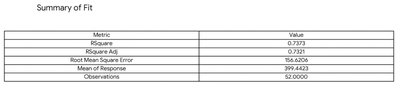
The Summary of Fit table provides key statistics about the regression model, including R2, RMSE, and the number of observations.

Parameter Estimates Table

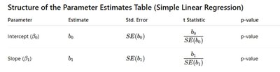
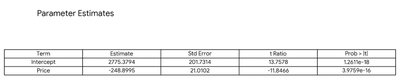
The Parameter Estimates Table summarizes the estimated coefficients, their standard errors, t-statistics, and p-values for hypothesis testing.

Inference for Regression Slope

Hypothesis Test for Slope

To determine if the explanatory variable significantly affects the response variable, we test:

• Null hypothesis (H0): (no linear relationship)

• Alternative hypothesis (Ha): (significant linear relationship)

The test statistic follows a t-distribution with degrees of freedom. If the p-value is less than the significance level (e.g., 0.05), we reject H0 and conclude that the slope is significant.

Confidence Interval for the Slope

A 95% confidence interval for the slope provides a range of plausible values for the true population slope .

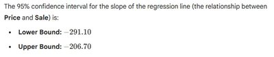
• Interpretation: We are 95% confident that for each $1 increase in price, the number of 12-pack cases sold decreases by between 206.7 and 291.1 on average.

Regression Assumptions

1. Linearity Assumption

The relationship between X and Y should be linear. This can be checked visually using a scatterplot.

2. Independence Assumption

The observations should be independent, often ensured by random sampling.

3. Equal Variance Assumption (Homoscedasticity)

The variance of residuals should be constant across all levels of X. This can be checked using residual plots.

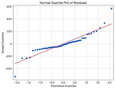
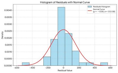
4. Normality Assumption

The residuals should be approximately normally distributed. This can be checked using a normal quantile plot and a histogram of residuals.

Evaluating Model Fit

• R2 (Coefficient of Determination): Indicates how well the model explains the variation in the response variable.

• RMSE (Root Mean Square Error): Measures the average magnitude of the residuals; lower values indicate a better fit.

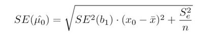
Confidence and Prediction Intervals for

Confidence Interval for the Estimated Mean Value of Y

Provides a range for the mean response at a given value of X:

Prediction Interval for an Individual Value of Y

Provides a range for an individual response at a given value of X:

• Prediction intervals are wider than confidence intervals because they account for both the uncertainty in estimating the mean and the additional variability of individual observations.

Example: For stores with price = $10, the 95% confidence interval for the mean number of 12-pack cases sold is between 238 and 334. The 95% prediction interval for an individual store is between 0 and 605.09.

Summary Table: Key Regression Output

Summary Table: Parameter Estimates

Conclusion

Simple linear regression provides a powerful framework for modeling and predicting the relationship between two quantitative variables. By checking assumptions, interpreting coefficients, and using inference, we can draw meaningful conclusions about the effect of one variable on another in a business context.