23–26. Loan problems The following initial value problems model the payoff of a loan. In each case, solve the initial value problem, for t≥0 graph the solution, and determine the first month in which the loan balance is zero.
B′(t) = 0.005B − 500, B(0) = 50,000
Verified step by step guidance
1
Identify the type of differential equation given: \( B'(t) = 0.005B - 500 \). This is a first-order linear ordinary differential equation.
Rewrite the equation in standard linear form: \( B'(t) - 0.005B = -500 \). This will help us apply the integrating factor method.
Calculate the integrating factor \( \mu(t) \) using the formula \( \mu(t) = e^{\int -0.005 \\ dt} = e^{-0.005t} \).
Multiply both sides of the differential equation by the integrating factor to get \( e^{-0.005t} B'(t) - 0.005 e^{-0.005t} B = -500 e^{-0.005t} \), which simplifies to \( \frac{d}{dt} \left( e^{-0.005t} B \right) = -500 e^{-0.005t} \).
Integrate both sides with respect to \( t \) to find \( e^{-0.005t} B(t) \), then solve for \( B(t) \). Use the initial condition \( B(0) = 50,000 \) to find the constant of integration.
Verified video answer for a similar problem:
This video solution was recommended by our tutors as helpful for the problem above
Video duration:
5m
Play a video:
0 Comments
Key Concepts
Here are the essential concepts you must grasp in order to answer the question correctly.
First-Order Linear Differential Equations
These are differential equations of the form B'(t) + p(t)B = q(t), where the solution involves finding an integrating factor. They model rates of change with linear dependence on the function itself, common in growth and decay problems like loan balances.
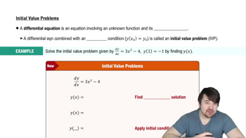
An IVP specifies the value of the unknown function at a particular point, here B(0) = 50,000. Solving an IVP means finding a unique solution that satisfies both the differential equation and the initial condition, ensuring the model fits the given scenario.
After solving the differential equation, the solution represents the loan balance over time. Determining when the balance reaches zero involves solving for t when B(t) = 0, which indicates the payoff time. Graphing helps visualize this behavior.

 Verified step by step guidance
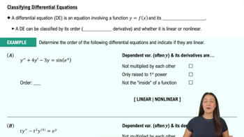
 07:39
07:39