Surfaces

Sections of Surfaces

In multivariable calculus, a surface can be described by a function of two variables, such as z = f(x, y). Each point (x, y) in the domain corresponds to a height value z, forming a surface above the xy-plane. To analyze the shape of a surface, we often examine sections—curves obtained by fixing one variable and varying the other.

• Section with y constant: Set y = c, then z = f(x, c) describes a curve in the xz-plane.

• Section with x constant: Set x = c, then z = f(c, y) describes a curve in the yz-plane.

• Contour (level curve): Set z = c, then f(x, y) = c describes a curve in the xy-plane where the surface has constant height.

Example: For z = x2 - y2, sections with y = 0, 1, 2 yield parabolas opening upwards, while sections with x = 0, 1, 2 yield parabolas opening downwards. The surface is a saddle (hyperbolic paraboloid).

Contour Plots

A contour plot (or level curve plot) is a projection of a surface onto the xy-plane, showing curves where the function takes constant values. These are widely used in topography and physics to represent surfaces such as hills or potential fields.

• Where contour lines are close together, the surface is steep.

• Where contour lines are far apart, the surface is relatively flat.

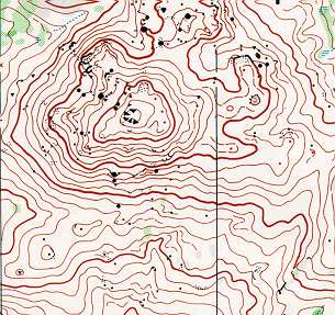
Example: The image above shows a contour plot, which could represent the surface z = x2 - y2 or a topographic map. Peaks, valleys, and saddle points can be identified by the arrangement of the contour lines.

Planes

The general equation of a plane in three dimensions is:

where (a, b, c) is a normal vector to the plane. Planes are the simplest surfaces and are characterized by linear equations in x, y, and z.

• Sections and contours of planes are straight, parallel lines.

• All points on a plane share the same normal vector.

Functions of Three Variables

Functions of three variables, such as T(x, y, z), can represent quantities like temperature in a room. Level surfaces (e.g., x2 + y2 + z2 = c) are called level surfaces or isosurfaces, generalizing the idea of contours to three dimensions.

Partial Derivatives and the Directional Derivative

Partial Derivatives

For a function f(x, y), the partial derivative with respect to x is found by treating y as a constant:

• : Rate of change of f in the x-direction.

• : Rate of change of f in the y-direction.

Example: If f(x, y) = x2y + x, then and .

Higher Order Partial Derivatives

Higher order partial derivatives are obtained by repeated differentiation. For example:

• means differentiate first with respect to y, then x.

Clairaut’s Theorem: If f is sufficiently smooth, mixed partial derivatives are equal: .

Taylor’s Theorem (Multivariable)

Taylor’s theorem allows us to approximate a function near a point using its derivatives. For f(x, y):

Directional Derivative

The directional derivative of f in the direction of a unit vector is:

This gives the rate of change of f in any specified direction.

The Gradient

Definition and Properties

The gradient of f(x, y) is the vector:

Key properties:

• Points in the direction of greatest increase of f.

• Magnitude gives the rate of fastest increase.

• Perpendicular to level curves (contours) of f.

Divergence, Curl, and Laplacian

Divergence

The divergence of a vector field is:

Measures the net rate of 'outflow' from a point.

Curl

The curl of a vector field is:

• (vector cross product with the del operator)

Measures the tendency to rotate about a point.

Laplacian

The Laplacian of a scalar function f is:

Appears in equations modeling diffusion, heat, and wave propagation.

Applications and Further Topics

• Double and triple integrals: Used to compute areas, volumes, mass, and other quantities over regions and volumes.

• Coordinate systems: Cylindrical and spherical coordinates are useful for problems with symmetry.

• Parameterization: Curves and surfaces can be described using parameters for integration and analysis.

• Vector fields: Functions assigning a vector to each point in space, important in physics and engineering.

Additional info: The image included is a contour plot, which visually represents level curves of a function of two variables. Such plots are essential in understanding the geometry of surfaces and are directly relevant to the study of multivariable calculus.