Graphs, Functions, and Models

Introduction to Functions & Their Graphs

Functions are fundamental mathematical objects that describe relationships between two sets, typically inputs (x-values) and outputs (y-values). In college algebra, functions are represented in various ways: equations, tables, graphs, and verbal descriptions.

• Definition of a Function: A function is a relation in which each input (x-value) has exactly one output (y-value).

• Domain: The set of all possible input values (x-values).

• Range: The set of all possible output values (y-values).

• Function Notation: Functions are often written as f(x) = expression, where y = f(x).

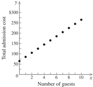
• Example: Cameron’s zoo membership cost can be modeled as $20x + $65 = y, where x is the number of guests and y is the total annual cost.

Representations of Functions

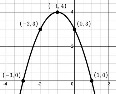
Functions can be described verbally, in tables, and graphically. For example, the function f(x) = -x^2 - 2x + 3 can be shown in all three forms.

• Verbal: The output equals the negative of the squared input, minus two times the input, plus three.

• Table: Shows specific input-output pairs.

• Graph: Visualizes the relationship between x and y.

Using Graphing Calculators

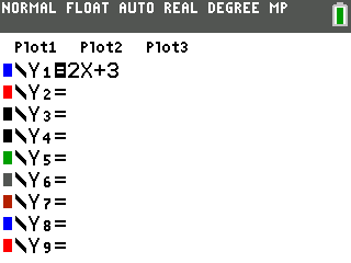
Graphing calculators like the TI-84/83 are essential tools for visualizing functions and analyzing their properties.

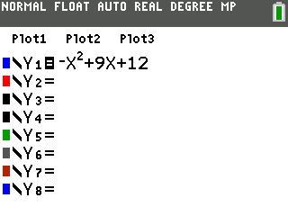
• Entering Functions: Use the Y= editor to input functions.

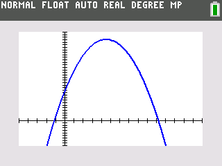
• Viewing Graphs: Adjust window settings to fit the graph.

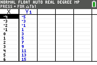
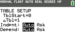
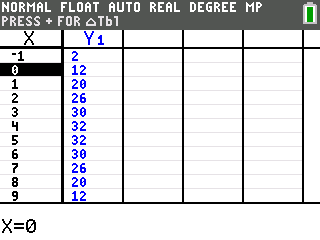
• Table Feature: View specific x and y values for the function.

Graphing Quadratic Functions

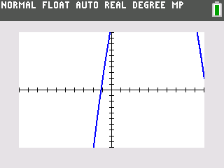
Quadratic functions have the form g(x) = ax^2 + bx + c and their graphs are parabolas. Adjusting the viewing window is often necessary to see the entire graph.

• Example: g(x) = -x^2 + 9x + 12

• Table Feature: Useful for finding specific values.

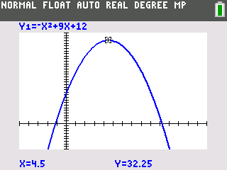
• Trace Feature: Allows you to find function values on the graph.

Domain and Range

The domain and range of a function describe the set of possible inputs and outputs. Restrictions may occur for rational or radical functions.

• Example: f(x) = \sqrt{x-2} has domain [2, ∞) because the square root is undefined for x < 2.

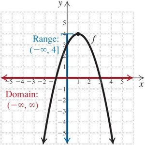
• Example: f(x) = -(x-1)^2 + 4 has domain (-∞, ∞) and range (-∞, 4].

Interval Notation

Interval notation is used to describe sets of numbers, especially domains and ranges. Parentheses indicate endpoints are not included; brackets indicate inclusion.

• Set-builder notation: {x | x < 5} is equivalent to interval notation (-∞, 5).

• Examples: (a) {x | x > 3} → (3, ∞) (b) {x | x ≤ -2} → (-∞, -2] (c) {x | -3 ≤ x ≤ -1} → [-3, -1] (d) {x | -4 < x < 0} → (-4, 0) (e) {x | 1 < x ≤ 4} → (1, 4]

Function Notation and Evaluation

Function notation provides a concise way to express and evaluate functions. To find f(a), substitute a for x in the function.

• Example: If h(x) = 2x^2 - x + 3, then h(-3) = 2(-3)^2 - (-3) + 3 = 18 + 3 + 3 = 24.

Multiplying Binomials (FOIL Method)

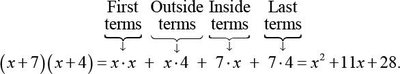
The FOIL method is used to multiply two binomials, applying the distributive property.

• Formula: (x + a)(x + b) = x^2 + (a + b)x + ab

• Example: (x + 7)(x + 4) = x^2 + 11x + 28

Linear Functions & Their Graphs

Graphing Linear Equations

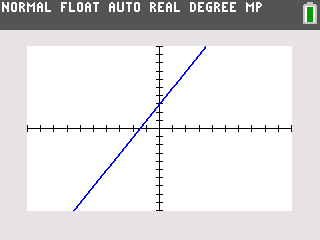
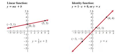
Linear functions have the form f(x) = mx + b, where m is the slope and b is the y-intercept. Their graphs are straight lines.

• Slope (m): The rate of change of y with respect to x.

• Y-intercept (b): The value of y when x = 0.

• Example: f(x) = 2x + 3

Finding Slopes and Intercepts

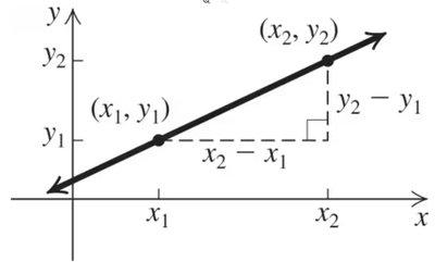
The slope of a line is calculated as the ratio of vertical change (rise) to horizontal change (run).

• Formula:

• X-intercept: Set y = 0 and solve for x.

• Y-intercept: Set x = 0 and solve for y.

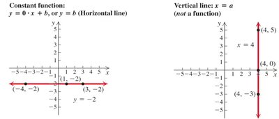
Horizontal and Vertical Lines

Horizontal lines have slope 0 and are functions. Vertical lines have undefined slope and are not functions.

• Horizontal line: y = b

• Vertical line: x = a

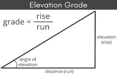
Applications of Slope

Slope is used to describe rates of change in real-world contexts, such as road grades, water usage, and population changes.

• Grade:

• Example: A 4% grade means a road rises 4 ft for every 100 ft horizontally.

Solving Linear Equations & Inequalities

Simplifying Linear Expressions

Combine like terms and use the distributive property to simplify expressions.

• Example: 3x - 5x + x = -x

• Distributive Property: a(b + c) = ab + ac

Solving Linear Equations

Use the addition and multiplication principles to isolate variables and solve equations.

• General Steps:

  1. Simplify each side.

  2. Collect variable terms on one side.

  3. Collect constant terms on the other side.

  4. Make the coefficient of the variable equal to 1.

  5. Check the solution.

• Example:

Solving Equations with Fractions

Multiply both sides by the least common denominator (LCD) to clear fractions.

• Example:

• Multiply both sides by 12 (LCD):

Solving Linear Inequalities

Apply the addition and multiplication principles for inequalities. Remember to reverse the inequality sign when multiplying or dividing by a negative number.

• Example:

• Interval notation: (-∞, -4]

Linear Application Models

Fixed Cost + Variable Rate Models

Many real-world scenarios involve a fixed cost plus a variable rate. These are modeled by linear functions.

• Formula:

• Example: Gym membership:

Percent Commission Models

Income models often include a base salary plus a percent commission on sales.

• Formula:

Final Amount After Percent Increase or Decrease

• Formula for Increase:

• Formula for Decrease:

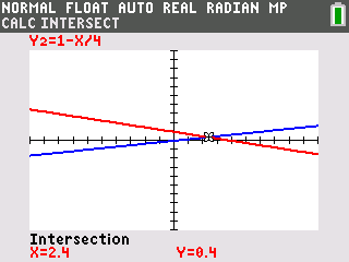
Systems of Linear Equations

Solving Systems of Equations

A system of equations consists of two or more equations considered simultaneously. The solution is the set of values that satisfy all equations.

• Methods: Graphing, substitution, and elimination.

• Example: and

• Solution: (2, -3)

Solving by Substitution

• Solve one equation for one variable.

• Substitute into the other equation.

• Solve for the remaining variable.

Solving by Elimination

• Align variables and constants.

• Multiply equations to eliminate a variable.

• Add or subtract equations.

• Solve for the remaining variable.

Applications of Systems

Systems of equations are used to solve real-world problems involving multiple constraints, such as break-even analysis, pricing, and resource allocation.

Tables

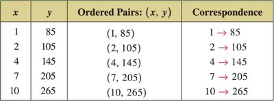
Ordered Pairs and Correspondence Table

This table shows the relationship between the number of guests and total admission cost, illustrating the concept of a function.

*Additional info: This study guide covers all major topics from Chapter 1 and part of Chapter 6, including functions, graphs, linear models, solving equations and inequalities, and systems of equations, as outlined in the college algebra syllabus.*