Matrices and Systems of Linear Equations

Introduction to Matrices

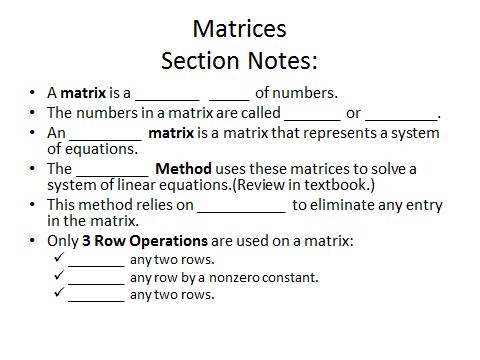
Matrices are essential tools in algebra for organizing and solving systems of linear equations. This section introduces the definition of matrices, their components, and their application in solving equations using systematic methods.

• Matrix: A rectangular array of numbers arranged in rows and columns.

• Entries: The numbers in a matrix are called elements or entries.

• Augmented Matrix: An augmented matrix represents a system of equations, including both the coefficients and constants.

Solving Systems with Matrices

Systems of linear equations can be rewritten in matrix form and solved using systematic procedures. The Gaussian Elimination Method is a standard approach that uses matrices to simplify and solve these systems.

• Gaussian Elimination Method: This method uses row operations to transform a matrix into a simpler form, making it easier to solve the corresponding system of equations.

• Row Operations: Only three types of row operations are allowed:

  • Interchange any two rows.

  • Multiply any row by a nonzero constant.

  • Add a multiple of one row to another row.

This method relies on elimination to remove variables and simplify the system.

Matrix Forms and Solution Types

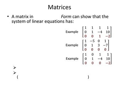
Transforming a matrix into Row Echelon Form (REF) or Reduced Row Echelon Form (RREF) reveals the nature of the solutions to the system.

• Row Echelon Form: A matrix is in REF if all nonzero rows are above any rows of all zeros, and each leading entry of a row is to the right of the leading entry of the row above it.

• Solution Types: The form of the matrix can indicate whether the system has a unique solution, infinitely many solutions, or no solution.

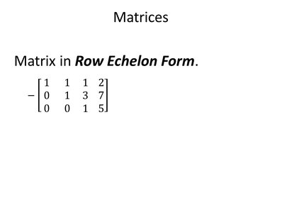
Row Echelon Form Example

The following is an example of a matrix in row echelon form, which is used to solve a system of equations by back-substitution:

• Example matrix:

Infinitely Many Solutions

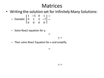
Some systems have infinitely many solutions, which can be identified when a row in the matrix reduces to all zeros. The solution set is written in terms of free variables.

• Example system:

• To solve:

  1. Solve the second row equation for y.

  2. Substitute y into the first row equation to solve for x.

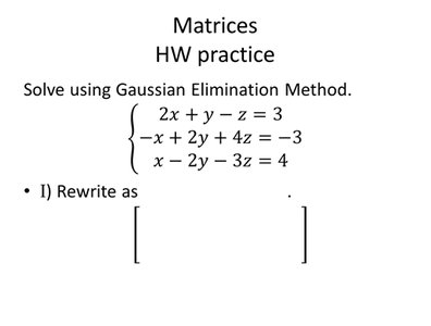
Gaussian Elimination Practice

To solve a system using the Gaussian Elimination Method, first rewrite the system as an augmented matrix, then perform row operations to reach row echelon form.

• Example system:

• Rewrite as an augmented matrix:

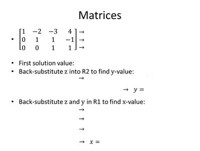
Back-Substitution and Solution

After reducing the matrix, use back-substitution to find the values of the variables.

• Example reduced matrix:

• Steps:

  1. Find the value of z from the last row.

  2. Substitute z into the second row to find y.

  3. Substitute y and z into the first row to find x.

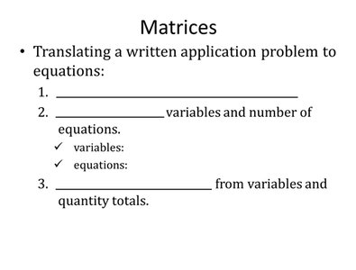
Translating Application Problems to Equations

Application problems can be solved using matrices by translating the problem into a system of equations.

• Identify what is being asked.

• Define variables and determine the number of equations needed.

• Write equations based on the relationships and totals given in the problem.

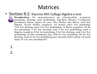
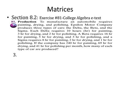
Application Example: Production Problem

Consider a production problem where different types of cars require different amounts of time for painting, drying, and polishing. The goal is to determine how many of each type of car can be produced given total available hours for each task.

• Let x, y, and z represent the number of Delta, Beta, and Sigma cars produced, respectively.

• Set up equations based on the time requirements and total available hours for each task.

• Solve the resulting system using matrices.

Summary Table: Row Operations

Key Formulas

• General form of a system of equations:

• Corresponding augmented matrix: