Lessons from Capital Markets History

Measuring Returns

Understanding how to measure investment returns is fundamental in financial accounting and corporate finance. Returns can be calculated in both dollar and percentage terms, and typically consist of two components: income (such as dividends) and capital gains (increase in asset value).

• Return: The profit earned from an investment, including both income and capital gains.

• Income Component: Cash received directly, such as dividends.

• Capital Gain: Increase in the value of the asset.

• Total Dollar Return: Sum of income and capital gain.

• Percentage Return: Total return divided by initial investment, expressed as a percentage.

• Formula:

• Alternative Formula:

• Example: If you invest $3,700 in 100 shares, receive $185 in dividends, and the shares appreciate to $4,033, your total dollar return is $518, and your total cash if sold is $4,218.

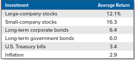
Historical Record of Returns

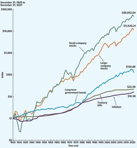
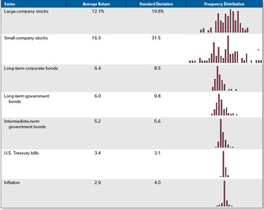
Historical data provides insight into the performance of various asset classes over time. Studies by Ibbotson and Sinquefield track returns for large-company stocks, small-company stocks, long-term corporate bonds, long-term government bonds, and Treasury bills.

• Large-company stocks: Represented by the S&P 500.

• Small-company stocks: Smallest 20% of NYSE companies.

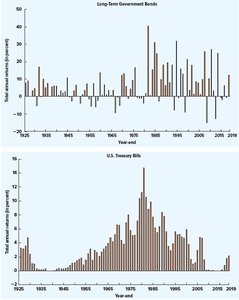
• Bonds: Corporate and government bonds with long maturities.

• Treasury bills: Short-term, risk-free government securities.

• Inflation: The rate at which prices increase over time, affecting real returns.

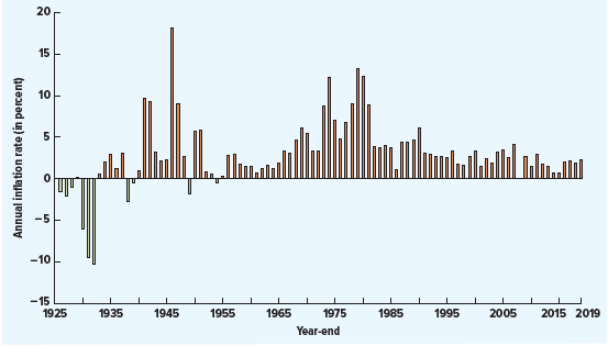
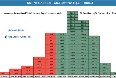
Year-by-Year Returns and Variability

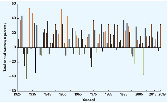
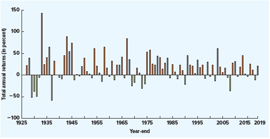
Annual returns for stocks and bonds fluctuate significantly, reflecting the inherent risk and volatility of these investments. Large-company stocks and small-company stocks show greater variability compared to bonds and Treasury bills.

• Volatility: The degree of variation in returns from year to year.

• Risk: Higher volatility implies higher risk.

• Example: S&P 500 returns ranged from highs of over 40% to lows below -40% in certain years.

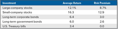
Average Returns and Risk Premiums

Average returns are calculated by summing annual returns and dividing by the number of years. Risk premium is the excess return earned by a risky asset over a risk-free asset, such as Treasury bills.

• Risk-Free Return: Return on Treasury bills, considered free of default risk.

• Risk Premium: Difference between average return on a risky asset and a risk-free asset.

• Example: Large-company stocks have an average return of 12.1% and a risk premium of 8.7% over Treasury bills.

Variability of Returns: Volatility, Variance, and Standard Deviation

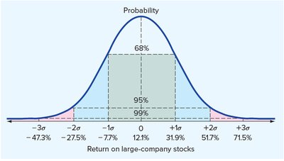
Volatility is quantified using variance and standard deviation, which measure the spread of returns around the average. The normal distribution is used to model the probability of returns falling within certain ranges.

• Variance: Average of squared deviations from the mean.

• Standard Deviation: Square root of variance, easier to interpret.

• Normal Distribution: Symmetric, bell-shaped curve defined by mean and standard deviation.

• Probability: 68% of returns fall within one standard deviation, 95% within two, 99% within three.

• Formula for Variance:

• Formula for Standard Deviation:

Capital Market Efficiency and Behavioral Finance

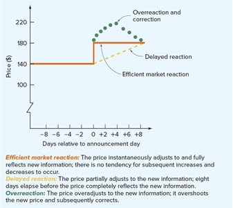
Capital market efficiency refers to the extent to which asset prices reflect all available information. The Efficient Market Hypothesis (EMH) posits that securities are fairly priced, and arbitrage corrects mispricing. Behavioral finance explores how psychological biases affect investor behavior and market outcomes.

• Efficient Market Hypothesis (EMH): Prices reflect all available information; all investments are zero NPV.

• Forms of Efficiency: Weak, semistrong, and strong, depending on the information reflected in prices.

• Behavioral Finance: Recognizes irrational behavior, psychological biases, and market anomalies.

• Key Principles: Prospect theory, mental accounting, overconfidence, framing, representativeness.

• Arbitrage: Corrects mispricing, but real-world limits exist.

Summary Table: Traditional vs. Behavioral Finance

Comparing traditional finance and behavioral finance highlights the role of rationality, market efficiency, and decision drivers.