 Back
BackAggregate Demand, Aggregate Supply, and Macroeconomic Fluctuations: Core Concepts in Macroeconomics
Study Guide - Smart Notes
 Tailored notes based on your materials, expanded with key definitions, examples, and context.
Recent Economic Activity and Labor Market Trends
Employment and Labor Force Dynamics
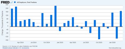
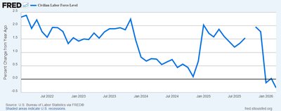
Recent data on employment and labor force participation provide insight into the health of the macroeconomy. The number of jobs added or lost each month, as well as changes in the labor force, are key indicators of economic performance.
Employment Change: The net change in jobs each month reflects the pace of economic expansion or contraction.
Labor Force Participation: The labor force includes all employed and unemployed individuals actively seeking work. A declining labor force can indicate demographic shifts, discouraged workers, or changes in immigration.
Aggregate Demand and Aggregate Supply (AD-AS) Model
Aggregate Demand (AD)
The aggregate demand curve shows the relationship between the overall price level and the quantity of real GDP demanded by households, firms, and the government. It is downward sloping due to three main effects:
Wealth Effect: Higher prices reduce the real value of money holdings, decreasing consumer spending.
Interest-Rate Effect: Higher prices lead to higher interest rates, reducing investment and consumption.
International Trade Effect: Higher domestic prices make exports less competitive, reducing net exports.
Shifts in Aggregate Demand can be caused by changes in monetary and fiscal policy, expectations of households and firms, and foreign economic conditions.
Aggregate Supply (AS)
The aggregate supply curve describes the relationship between the price level and the quantity of goods and services firms are willing to produce.
Long-Run Aggregate Supply (LRAS): In the long run, real GDP is determined by resources (labor, capital, technology), not the price level. The LRAS is vertical at the economy's potential output.
Short-Run Aggregate Supply (SRAS): In the short run, the SRAS is upward sloping because input prices (like wages) adjust more slowly than output prices, and some firms are slow to adjust their own prices.
Shifts in Aggregate Supply
Increases in Labor Force or Capital Stock: Shift SRAS to the right (more output at every price level).
Technological Change: Improves productivity, shifting SRAS to the right.
Expected Future Prices: If firms expect higher future prices, SRAS shifts left.
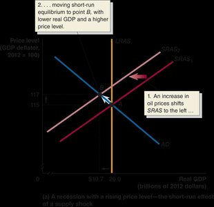
Supply Shocks: Sudden increases in input costs (e.g., oil) shift SRAS left, causing stagflation.
Macroeconomic Equilibrium
Equilibrium occurs where AD, SRAS, and LRAS intersect. In the long run, the economy returns to potential GDP, but in the short run, shocks can cause output and prices to deviate from potential.
Supply Shocks and Stagflation
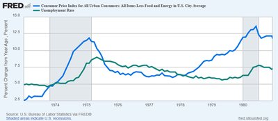
Supply shocks, such as oil price spikes or natural disasters, can shift SRAS left, leading to higher inflation and unemployment—a phenomenon known as stagflation.
Case Study: The COVID-19 Recession
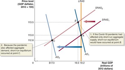
The 2020 recession was unique in that both aggregate demand and aggregate supply declined. Business closures reduced output and employment, while consumer and investment spending fell sharply. The result was a significant drop in real GDP and the price level.
Measuring Economic Activity: GDP and Its Components
Gross Domestic Product (GDP)
GDP measures the market value of all final goods and services produced within a country in a given period. It can be measured by total production or total income, as every dollar spent is income for someone else.
Expenditure Approach:
Final Goods: Only final goods are counted to avoid double counting; intermediate goods are excluded.
Real vs. Nominal GDP
Nominal GDP: Measured at current prices.
Real GDP: Adjusted for inflation, measured at base-year prices.
GDP Deflator:
Limitations of GDP
Does not include the underground economy or non-market activities.
Does not account for environmental harm or the value of leisure.
Disposable Personal Income
Disposable personal income is personal income minus taxes, representing income available for spending or saving.
Unemployment and Inflation
Measuring Unemployment
Unemployment Rate:
Labor Force: Employed + Unemployed (actively seeking work).
Not in Labor Force: Retirees, homemakers, students, etc.
Discouraged Workers: Not actively seeking work due to lack of available jobs.
Types of Unemployment
Frictional: Short-term, matching workers with jobs.
Structural: Mismatch between skills and job requirements.
Cyclical: Due to economic downturns.
Measuring Inflation
Consumer Price Index (CPI): Measures average price changes for a basket of goods and services.
Inflation Rate: Percentage change in CPI.
Problems Caused by Inflation
Reduces purchasing power if incomes do not keep pace.
Menu costs: Costs of changing prices.
Unanticipated inflation can hurt lenders and those on fixed incomes.
Distributional Effects of Inflation
Hurts those whose incomes do not rise with prices, especially people on fixed incomes.
Unexpected inflation benefits borrowers at the expense of lenders.
Long-Term Economic Growth
Real GDP per Capita
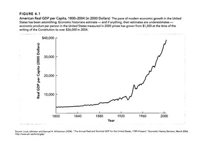
Real GDP per capita is the best measure of living standards over time and across countries, as it adjusts for population size.
Determinants of Economic Growth
Physical Capital: Factories, machinery, and infrastructure.
Human Capital: Education, skills, and health of the workforce.
Technology: Innovations and improvements in production methods.
The Market for Loanable Funds
Interest Rates and Investment
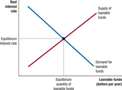
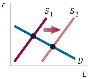
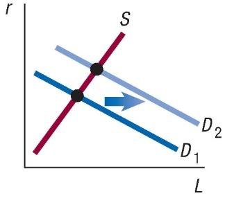
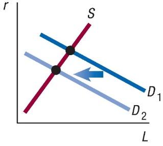
The market for loanable funds determines the real interest rate, balancing the supply of savings with the demand for investment funds.
Supply: Provided by households and foreign investors; increases with higher interest rates.
Demand: Driven by firms, government, and households; decreases with higher interest rates.
Shifts in Loanable Funds Market
Event | Curve Shift | Effect on Equilibrium |
|---|---|---|
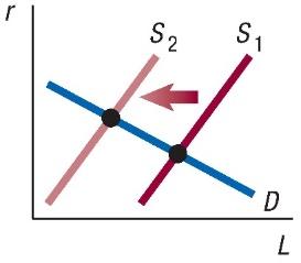
Increase in government deficit | Supply shifts left | Interest rate up, investment down |
Increase in desire to consume today | Supply shifts left | Interest rate up, investment down |
Tax benefits for saving | Supply shifts right | Interest rate down, investment up |
Expected future profits rise | Demand shifts right | Interest rate up, investment up |
Increase in corporate taxes | Demand shifts left | Interest rate down, investment down |
Business Cycles and Macroeconomic Fluctuations
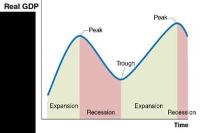
The Business Cycle
The business cycle consists of alternating periods of economic expansion and recession. Peaks mark the end of expansions, and troughs mark the end of recessions.
Aggregate Expenditure and Output
Aggregate expenditures (AE) represent total spending in the economy. When AE equals GDP, the economy is in equilibrium. Deviations lead to changes in inventories, prompting firms to adjust production.
If... | Then... | And... |
|---|---|---|
Aggregate expenditure equals GDP | Inventories unchanged | Economy in equilibrium |
Aggregate expenditure less than GDP | Inventories rise | GDP and employment decrease |
Aggregate expenditure greater than GDP | Inventories fall | GDP and employment increase |
The Multiplier Effect
The multiplier quantifies how an initial change in autonomous spending leads to a larger change in equilibrium GDP.
Formula: , where MPC is the marginal propensity to consume.
Example: If MPC = 0.75, then .
A $200 billion increase in investment spending can ultimately increase GDP by $800 billion if the multiplier is 4.
Determinants of Key Macroeconomic Variables
Consumer Spending
Disposable income (after taxes)
Household wealth
Expected future income
Price level
Interest rates
Planned Investment
Expectations of future profitability
Interest rates
Taxes
Cash flow
Government Purchases
Federal spending rises during downturns and military escalations
State/local spending may fall during downturns due to balanced budget requirements
Net Exports
Relative inflation rates
Relative GDP growth rates
Exchange rates
