 Back
BackAggregate Demand and Aggregate Supply Analysis: Study Guide
Study Guide - Smart Notes
 Tailored notes based on your materials, expanded with key definitions, examples, and context.
Aggregate Demand and Aggregate Supply Analysis
Introduction
This chapter explores the aggregate demand and aggregate supply (AD-AS) model, a fundamental framework in macroeconomics used to explain fluctuations in real GDP, employment, and the price level. The AD-AS model helps us understand both short-run and long-run economic dynamics, including the effects of policy interventions and external shocks.
Aggregate Demand
Components of Aggregate Demand
Aggregate demand (AD) represents the total quantity of goods and services demanded across the economy at different price levels. It is composed of:
Consumption (C): Spending by households on goods and services.
Investment (I): Spending by firms on capital goods and by households on new housing.
Government Purchases (G): Expenditures by government agencies.
Net Exports (NX): Exports minus imports.
The aggregate demand equation is:
The Aggregate Demand Curve
The AD curve shows the relationship between the price level and the quantity of real GDP demanded. It slopes downward due to three main effects:
Wealth Effect: As price levels rise, the real value of household wealth declines, reducing consumption.
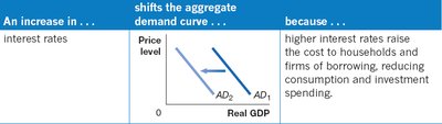
Interest-Rate Effect: Higher price levels increase the demand for money, raising interest rates and discouraging investment.
International-Trade Effect: Higher U.S. price levels make exports more expensive and imports cheaper, reducing net exports.
Movements Along vs. Shifts of the AD Curve
Movement Along: Caused by changes in the price level, holding other factors constant.
Shift: Caused by changes in components of real GDP (C, I, G, NX) or other external variables.
Variables That Shift the Aggregate Demand Curve
Several factors can shift the AD curve:
Monetary Policy: Changes in interest rates by the Federal Reserve affect investment and consumption.
Fiscal Policy: Changes in government purchases or taxes affect aggregate demand.
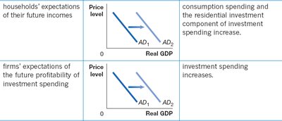
Expectations: Optimism or pessimism among households and firms can alter consumption and investment.
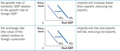
Foreign Income and Exchange Rates: Changes in foreign incomes or the value of the dollar affect net exports.
Variable | Effect on AD Curve | Reason |
|---|---|---|
Interest rates | Shift left | Higher rates reduce consumption and investment |
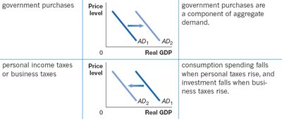
Government purchases | Shift right | Government spending increases aggregate demand |
Personal/business taxes | Shift left | Higher taxes reduce consumption and investment |
Household/firms expectations | Shift right | Optimism increases spending |
Foreign income/exchange rate | Shift left | Higher dollar reduces exports, increases imports |
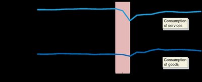
Aggregate Demand During the 2020 Recession
The COVID-19 recession saw significant changes in the components of aggregate demand:
Consumption of services fell sharply, while consumption of goods was less affected.
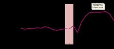
Residential investment increased after an initial drop.
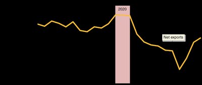
Net exports declined as exports fell and imports rose.
Aggregate Supply
Definition and Types
Aggregate supply (AS) is the total quantity of goods and services firms are willing and able to produce at different price levels. It is analyzed in both the short run and long run:
Long-Run Aggregate Supply (LRAS): Shows the relationship between price level and real GDP supplied in the long run, determined by resources, technology, and capital stock.
Short-Run Aggregate Supply (SRAS): Shows the relationship in the short run, where prices of inputs may be sticky.
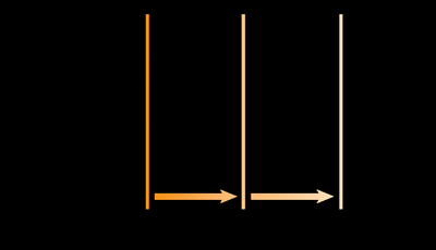
The Long-Run Aggregate Supply Curve
LRAS is vertical at the level of potential or full-employment GDP, which advances each year as resources and technology improve. LRAS does not depend on the price level.
The Short-Run Aggregate Supply Curve
SRAS is upward sloping because:
Sticky Wages and Prices: Contracts and menu costs make wages and prices slow to adjust.
Slow Wage Adjustments: Firms are reluctant to cut wages and adjust them infrequently.
Menu Costs: Firms incur costs when changing prices, making them slow to respond to demand changes.
Movements Along vs. Shifts of the SRAS Curve
Movement Along: Caused by changes in the price level, holding other factors constant.
Shift: Caused by changes in factors affecting production, such as labor force, capital stock, productivity, or input prices.
Variables That Shift the SRAS Curve
Several factors can shift the SRAS curve:
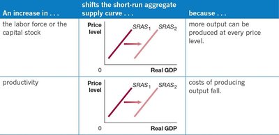
Labor Force or Capital Stock: Increases allow more output at every price level.
Productivity: Higher productivity reduces production costs.
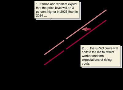
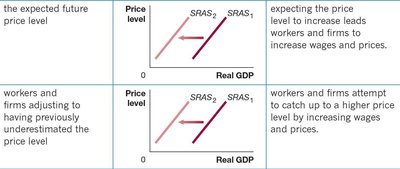
Expected Future Price Level: If workers and firms expect higher prices, they adjust wages and prices upward.
Adjustment to Underestimated Price Level: Workers and firms catch up to higher prices by increasing wages and prices.
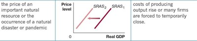
Supply Shocks: Unexpected events (e.g., natural disasters, pandemics) raise input costs or force closures.
Variable | Effect on SRAS Curve | Reason |
|---|---|---|
Labor force/capital stock | Shift right | More output at every price level |
Productivity | Shift right | Lower production costs |
Expected future price level | Shift left | Higher expected prices lead to higher wages/prices |
Adjustment to underestimated price level | Shift left | Wages/prices catch up to higher price level |
Supply shock | Shift left | Higher input costs or closures |
Macroeconomic Equilibrium
Short-Run and Long-Run Equilibrium
Macroeconomic equilibrium occurs where the AD and AS curves intersect. In the short run, equilibrium can deviate from potential GDP due to sticky prices and wages. In the long run, the economy tends to return to potential GDP as prices and wages adjust.
Summary Table: AD and SRAS Shifters
Factor | AD/SRAS | Direction | Explanation |
|---|---|---|---|
Interest rates | AD | Left | Higher rates reduce spending |
Government purchases | AD | Right | Increase in demand |
Taxes | AD | Left | Reduce consumption/investment |
Expectations | AD | Right | Increase spending |
Foreign income/exchange rate | AD | Left | Reduce net exports |
Labor force/capital stock | SRAS | Right | Increase output |
Productivity | SRAS | Right | Lower costs |
Expected price level | SRAS | Left | Higher wages/prices |
Supply shock | SRAS | Left | Higher input costs |
Conclusion
The AD-AS model is essential for understanding macroeconomic fluctuations and the effects of policy interventions. By analyzing the factors that shift aggregate demand and supply, economists can predict and respond to changes in real GDP, employment, and the price level.
