Aggregate Demand and Aggregate Supply Analysis – Macroeconomics Study Notes

Study Guide - Smart Notes

Tailored notes based on your materials, expanded with key definitions, examples, and context.

Aggregate Demand and Aggregate Supply Model

Introduction to the AD-AS Model

The Aggregate Demand and Aggregate Supply (AD-AS) model is a fundamental framework in macroeconomics used to explain short-run fluctuations in real GDP and the price level. The intersection of the aggregate demand curve and the short-run aggregate supply curve determines the equilibrium level of real GDP and the price level in the short run.

Aggregate Demand (AD) Curve: Shows the relationship between the price level and the quantity of real GDP demanded by households, firms, and the government.
Short-Run Aggregate Supply (SRAS) Curve: Shows the relationship in the short run between the price level and the quantity of real GDP supplied by firms.
Long-Run Aggregate Supply (LRAS) Curve: Shows the relationship in the long run between the price level and the quantity of real GDP supplied, which is determined by resources and technology.

Equation for GDP:

where is GDP, is consumption, is investment, is government purchases, and is net exports.

Aggregate Demand (AD)

Why the Aggregate Demand Curve is Downward Sloping

The AD curve slopes downward due to three main effects:

Wealth Effect: A lower price level increases the real value of household wealth, leading to higher consumption and greater demand for goods and services.
Interest-Rate Effect: A lower price level reduces the need for money holdings, leading to lower interest rates and increased investment spending.
International-Trade Effect: A lower domestic price level makes exports more attractive and imports less attractive, increasing net exports.

Movements Along vs. Shifts of the AD Curve

A change in the price level causes a movement along the AD curve. Changes in other variables (C, I, G, NX) shift the AD curve.

Determinants of Aggregate Demand

Events that change consumption, investment, government purchases, or net exports (other than the price level) will shift the AD curve.

Consumption (C): Changes in consumer confidence, taxes, or wealth.
Investment (I): Changes in interest rates, business expectations, or tax incentives.
Government Purchases (G): Changes in federal, provincial, or municipal spending.
Net Exports (NX): Changes in foreign demand, exchange rates, or relative growth rates.

Table: Variables That Shift the Aggregate Demand Curve

Variable	Effect on AD Curve	Reason
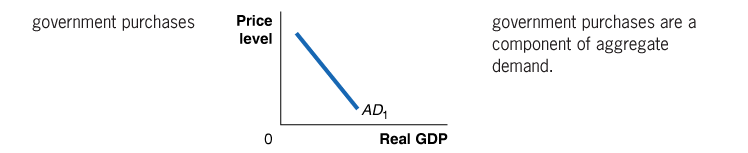
Government purchases	Shifts right if increased	Government purchases are a component of aggregate demand.
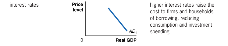
Interest rates	Shifts left if increased	Higher interest rates raise the cost to firms and households of borrowing, reducing consumption and investment spending.
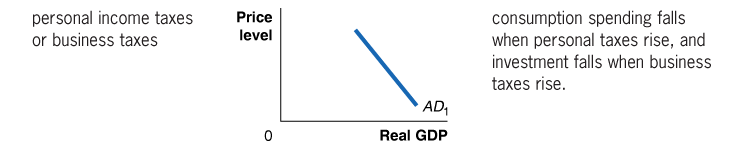
Personal income taxes or business taxes	Shifts left if increased	Consumption spending falls when personal taxes rise, and investment falls when business taxes rise.
Households’ expectations of their future incomes	Shifts right if increased	Consumption spending increases.
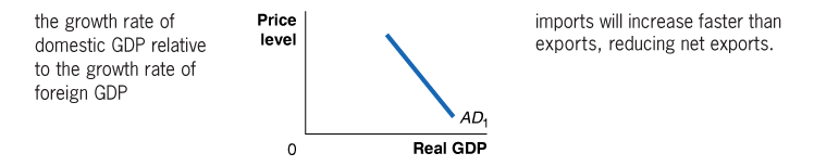
Growth rate of domestic GDP relative to foreign GDP	Shifts left if domestic grows faster	Imports will increase faster than exports, reducing net exports.
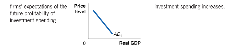
Firms’ expectations of future profitability of investment spending	Shifts right if increased	Investment spending increases.
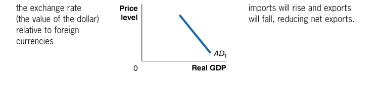
Exchange rate (value of dollar relative to foreign currencies)	Shifts left if dollar appreciates	Imports will rise and exports will fall, reducing net exports.

Government purchases and AD curve Interest rates and AD curve Personal income taxes or business taxes and AD curve Households’ expectations of future incomes and AD curve Growth rate of domestic GDP relative to foreign GDP and AD curve Firms’ expectations of future profitability of investment spending and AD curve Exchange rate and AD curve

Aggregate Supply (AS)

Short-Run vs. Long-Run Aggregate Supply

The aggregate supply curve shows the total quantity of goods and services that firms produce and sell at any given price level.

Short-Run Aggregate Supply (SRAS): Upward sloping because some prices and wages are sticky in the short run.
Long-Run Aggregate Supply (LRAS): Vertical at potential GDP (full-employment output), determined by resources and technology.

Why the SRAS Curve is Upward Sloping

Sticky-Wage Theory: Nominal wages are slow to adjust, so higher prices increase profitability and output.
Sticky-Price Theory: Some prices are slow to adjust due to menu costs, so unexpected price changes affect output.

SRAS Equation:

where is output, is natural rate of output, is actual price level, is expected price level, and measures responsiveness.

Determinants of Short-Run Aggregate Supply

Variables that shift the SRAS curve include changes in the labor force, capital stock, productivity, expected future price level, and prices of important natural resources.

Variable	Effect on SRAS Curve	Reason
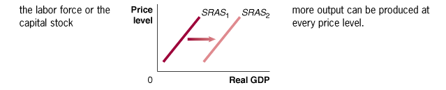
Labor force or capital stock	Shifts right if increased	More output can be produced at every price level.
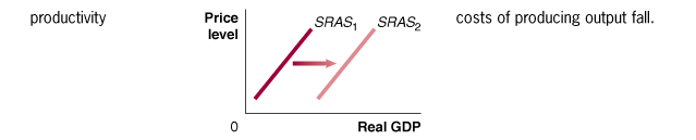
Productivity	Shifts right if increased	Costs of producing output fall.
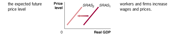
Expected future price level	Shifts left if increased	Workers and firms increase wages and prices.
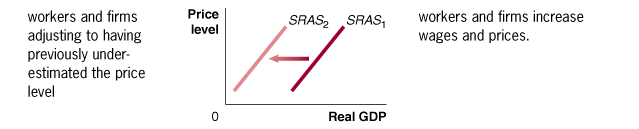
Workers and firms adjusting to previously underestimated price level	Shifts left	Workers and firms increase wages and prices.
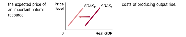
Expected price of an important natural resource	Shifts left if increased	Costs of producing output rise.

Labor force or capital stock and SRAS curve Productivity and SRAS curve Expected future price level and SRAS curve Workers and firms adjusting to underestimated price level and SRAS curve Expected price of an important natural resource and SRAS curve

Macroeconomic Equilibrium

Short-Run and Long-Run Equilibrium

Macroeconomic equilibrium occurs where the AD, SRAS, and LRAS curves intersect. In the short run, output can deviate from potential GDP, but in the long run, the economy returns to potential GDP as expectations adjust.

Short-Run Equilibrium: Intersection of AD and SRAS; output may be above or below potential.
Long-Run Equilibrium: Intersection of AD, SRAS, and LRAS; output equals potential GDP, and unemployment is at its natural rate.

Adjustment Mechanisms

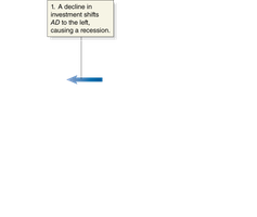
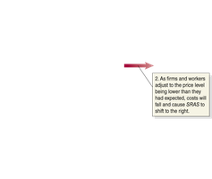
If AD decreases, the economy enters a recession in the short run, but SRAS shifts right over time, restoring potential GDP at a lower price level.
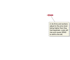
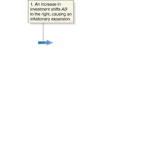
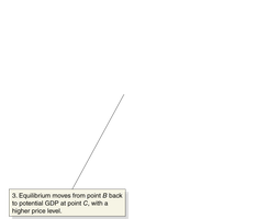
If AD increases, the economy experiences an expansion in the short run, but SRAS shifts left over time, restoring potential GDP at a higher price level.
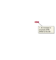
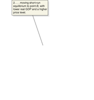
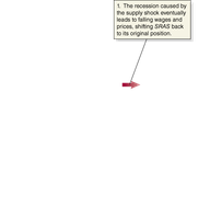
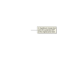
Supply shocks (e.g., oil price spikes) shift SRAS left, causing stagflation (recession + inflation). Over time, SRAS shifts back as wages and prices adjust.

AD decrease and macroeconomic equilibrium adjustment AD increase and macroeconomic equilibrium adjustment Supply shock and macroeconomic equilibrium adjustment

Macroeconomic Schools of Thought

Keynesian Model

Emphasizes the role of aggregate demand in causing short-run fluctuations in output and employment. Prices and wages are sticky, so government intervention can help stabilize the economy.

Monetarist Model

Focuses on the role of the money supply in influencing real output. Advocates for a constant growth rate of the money supply to avoid economic fluctuations.

New Classical Model

Emphasizes rational expectations and the importance of correct price and wage expectations. Fluctuations are minimized if expectations are accurate.

Real Business Cycle Model

Attributes business cycles to real (not monetary) shocks, such as changes in productivity. Assumes prices and wages adjust quickly, so only real shocks affect output.

Marxist Critique

Karl Marx argued that capitalism would eventually collapse due to inherent exploitation and crises, to be replaced by a communist system controlled by workers.

Additional info: These notes synthesize and expand upon the provided slides and images, ensuring a comprehensive and academically rigorous overview of the AD-AS model and its macroeconomic implications.