Aggregate Demand Curve: Derivation and Effects

Introduction to Aggregate Demand (AD)

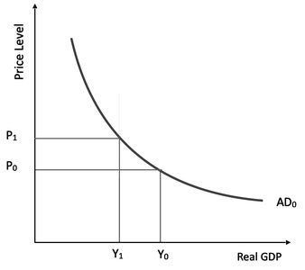
The aggregate demand curve illustrates the relationship between the price level and the total quantity of real GDP demanded in an economy. Unlike market demand curves, the AD curve is downward sloping due to macroeconomic effects rather than individual price changes.

• Wealth Effect: When the price level rises, the real value of money holdings decreases, reducing private sector wealth and consumption expenditure (C), which lowers aggregate expenditure (AE).

• Net Export Effect: A higher domestic price level makes domestic goods less competitive internationally, decreasing exports and increasing imports, thus reducing net exports (NX) and AE.

• Additional info: A third effect related to interest rates is discussed in later chapters.

Key Points

• Price Level Increase: Leads to a decrease in real wealth, consumption, net exports, and aggregate expenditure.

• Price Level Decrease: Increases real wealth, consumption, net exports, and aggregate expenditure.

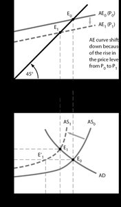
• Movement Along AD Curve: Caused by exogenous changes in the price level, shifting AE and changing equilibrium GDP.

Aggregate Demand Curve: Shifts

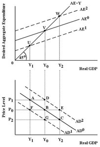
Shifts Due to Autonomous Expenditure

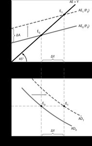
Changes in autonomous expenditure (such as investment, government spending, or exports) shift the AD curve horizontally. For a given price level, an increase in autonomous expenditure shifts the AE curve vertically, resulting in a new equilibrium GDP.

• AD Shocks: Any event that changes autonomous expenditure causes a shift in the AD curve.

• Simple Multiplier (SM): The horizontal shift in AD is given by .

• Example: A $100 million increase in investment expenditure shifts the AD curve to the right by the multiplier effect.

Aggregate Supply Curve

Short-Run Aggregate Supply (AS)

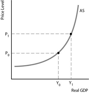
The aggregate supply curve shows the relationship between the price level and the quantity of real GDP supplied, holding technology and factor prices constant. The AS curve is upward sloping because unit costs rise as output increases, due to diminishing productivity of additional inputs.

• Low Output: Firms have excess capacity, so costs do not rise quickly.

• High Output: Unit costs increase rapidly as firms use less productive inputs.

• AS Shocks: Increases in input prices or decreases in technology shift the AS curve upward.

Short-Run Macroeconomic Equilibrium

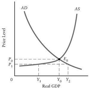
AD–AS Equilibrium

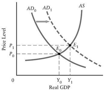
Macroeconomic equilibrium occurs at the intersection of the AD and AS curves, determining the equilibrium price level and real GDP.

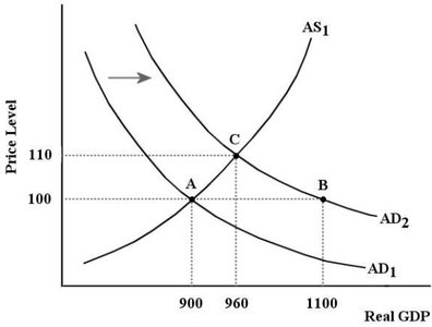
• AD Shocks: An increase in autonomous expenditure shifts AD right, raising both price level and real GDP.

• AS Shocks: Changes in firms' costs or technology shift AS, affecting price level and real GDP in opposite directions.

• Multiplier Effect: The steeper the AS curve, the greater the price effect and the smaller the output effect.

Macroeconomic Shocks and Their Effects

Types of Shocks

• AD Shocks: Caused by changes in autonomous expenditure (e.g., investment, government spending, exports).

• AS Shocks: Caused by changes in input prices (e.g., wages, oil prices) or technology.

• Combined Effects: Many real-world events affect both AD and AS, with the overall impact depending on the relative strength of each effect.

Exercises: Application of AD and AS Concepts

Wealth Effect and Net Export Effect

• Wealth Effect:

  • If the price level rises, real value of money holdings decreases.

  • If the price level falls, real value of money holdings increases.

  • Increases in real wealth lead to increases in autonomous consumption and AE shifts up.

  • Decreases in real wealth lead to decreases in autonomous consumption and AE shifts down.

• Net Export Effect:

  • If the price level increases, Canadian products become less internationally competitive, exports decrease, imports increase.

  • If the price level decreases, Canadian products become more internationally competitive, exports increase, imports decrease.

AD Curve Derivation and Shifts

• Movement Along AD Curve: Caused by exogenous changes in the price level.

• AD Curve Shifts: Caused by changes in autonomous expenditure, with the magnitude determined by the simple multiplier.

Comparing Economies: Multiplier Effect

• Economy A (higher marginal propensity to consume, lower tax and import rates) has a larger multiplier and greater AD curve shift in response to a common shock than Economy B.

• Multiplier formula:

Macroeconomic Impact Table

The following table summarizes the effects of various macroeconomic events on aggregate demand, aggregate supply, equilibrium price level, and equilibrium GDP:

Multiplier Calculations

• Simple Multiplier (SM):

• Multiplier Effect: The actual multiplier may be less than the simple multiplier if the price level changes.

Summary Table: AD and AS Shocks

Conclusion

The AD and AS model is central to understanding short-run macroeconomic equilibrium. Changes in the price level, autonomous expenditure, input prices, and technology all affect real GDP and the price level through shifts and movements in the AD and AS curves. The multiplier effect quantifies the impact of changes in autonomous expenditure, and the relative steepness of the AS curve determines the balance between price and output effects.