Aggregate Demand and Aggregate Supply

Aggregate Demand (AD)

Aggregate demand is the total quantity of final goods and services produced in an economy that all sectors (households, businesses, government, and foreigners) plan to buy at each price level. It is a central concept in macroeconomics, reflecting the overall demand for real GDP.

• Formula: where C is consumption, I is investment, G is government expenditure, X is exports, and M is imports.

• Main influences on aggregate demand:

  • The price level

  • Expectations about future income, inflation, and profits

  • Fiscal policy (taxes, government spending, transfer payments)

  • Monetary policy (interest rates, money supply)

  • The world economy (exchange rates, foreign income)

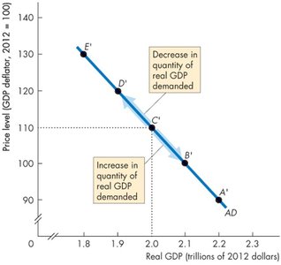
The Aggregate Demand Curve

The aggregate demand curve shows the relationship between the quantity of real GDP demanded and the price level. It is downward sloping due to the wealth effect and substitution effects.

• Wealth effect: As the price level falls, the real value of wealth increases, leading to higher consumption.

• Substitution effects: As the domestic price level falls, domestic goods become relatively cheaper than foreign goods, increasing exports and decreasing imports.

Main Influences on Aggregate Demand

Aggregate demand can shift due to changes in expectations, fiscal and monetary policy, and the world economy.

• Expectations: Higher expected future income, inflation, or profits increase aggregate demand.

• Fiscal policy: Tax cuts or increased government spending raise aggregate demand.

• Monetary policy: Lower interest rates or increased money supply boost aggregate demand.

• World economy: A lower exchange rate or higher foreign income increases demand for exports, raising aggregate demand.

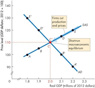
Short-Run Macroeconomic Equilibrium

Short-run equilibrium occurs where the aggregate demand curve (AD) intersects the short-run aggregate supply curve (SAS). At this point, the quantity of real GDP demanded equals the quantity supplied at the current price level.

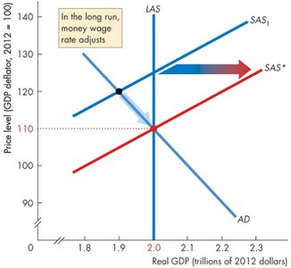
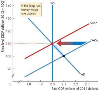
Long-Run Macroeconomic Equilibrium

Long-run equilibrium is achieved when real GDP equals potential GDP, at the intersection of the AD and long-run aggregate supply (LAS) curves. Adjustments in the money wage rate shift the SAS curve until equilibrium is restored at potential GDP.

• If the economy is below full employment, the money wage falls, shifting SAS rightward.

• If the economy is above full employment, the money wage rises, shifting SAS leftward.

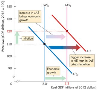
Inflation and Economic Growth in the AS-AD Model

If aggregate demand increases faster than long-run aggregate supply, the result is inflation. Economic growth occurs when both AD and LAS shift rightward, but inflation arises if AD shifts more rapidly than LAS.

The Business Cycle and the AS-AD Model

The business cycle is explained by fluctuations in aggregate demand and short-run aggregate supply, with the money wage rate adjusting slowly. Key concepts include:

• Inflationary gap: Real GDP exceeds potential GDP (above full employment).

• Recessionary gap: Potential GDP exceeds real GDP (below full employment).

• Full-employment equilibrium: Real GDP equals potential GDP.

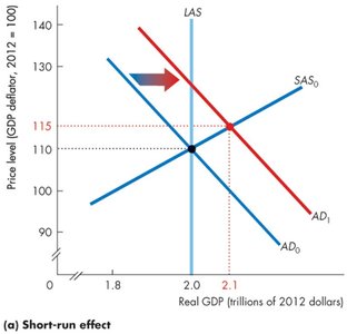
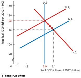
Fluctuations in Aggregate Demand and Supply

Short-run and long-run effects of changes in aggregate demand and supply are central to understanding macroeconomic fluctuations.

• Increase in aggregate demand (short run): AD shifts right, raising output and prices (inflationary gap).

• Increase in aggregate demand (long run): Money wage rises, SAS shifts left, and real GDP returns to potential GDP at a higher price level.

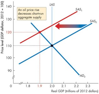
• Decrease in short-run aggregate supply: For example, a rise in oil prices shifts SAS left, causing stagflation (higher prices, lower output).

Main Schools of Macroeconomic Thought

• Classical: The economy is self-regulating and always at full employment.

• Keynesian: The economy often needs active fiscal and monetary policy to achieve full employment.

• Monetarist: The economy is self-regulating if monetary policy is stable and predictable.

Expenditure Multipliers

The Two-Way Link Between Aggregate Expenditure and Real GDP

The Keynesian model analyzes the economy in the very short run when prices are fixed. Aggregate expenditure (AE) determines real GDP, and real GDP influences components of AE, especially consumption and imports.

• Formula:

• When real GDP increases, aggregate expenditure increases (and vice versa).

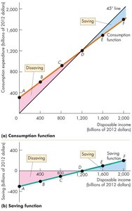
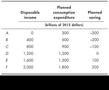
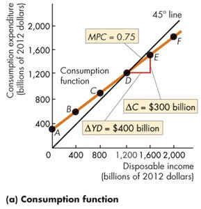
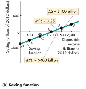
Consumption and Savings Plans

Disposable income (YD) is the main determinant of consumption and saving. It is defined as aggregate income minus net taxes:

• Formula:

• Disposable income is either consumed or saved:

• The consumption function shows the relationship between consumption and disposable income.

• The saving function shows the relationship between saving and disposable income.

Marginal Propensities to Consume and Save

The marginal propensity to consume (MPC) is the fraction of an increase in disposable income that is spent on consumption. The marginal propensity to save (MPS) is the fraction saved.

• Formula for MPC:

• Formula for MPS:

• MPC + MPS = 1

Aggregate Planned Expenditure, Import Function, AE Curve, and Equilibrium Expenditure

Aggregate planned expenditure (AE) is the total amount of spending planned at each level of real GDP. The AE curve graphs this relationship. Imports are primarily influenced by real GDP in the short run, and the marginal propensity to import measures the fraction of additional income spent on imports.

• Autonomous expenditure: Components of AE not influenced by real GDP (investment, government spending, exports).

• Induced expenditure: Components of AE that change with real GDP (consumption, imports).

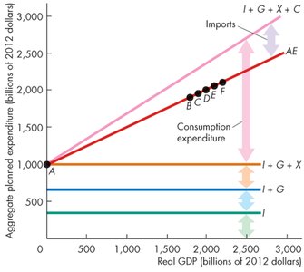
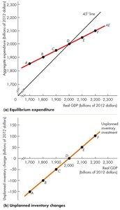
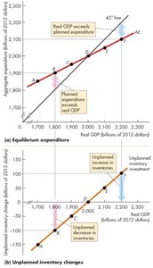
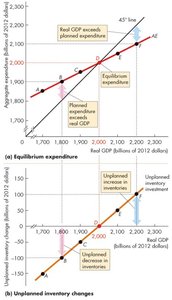
Equilibrium Expenditure

Equilibrium expenditure occurs where aggregate planned expenditure equals real GDP. At this point, there are no unplanned changes in inventories.

• If planned expenditure exceeds real GDP, inventories fall, firms increase production, and real GDP rises.

• If planned expenditure is less than real GDP, inventories rise, firms decrease production, and real GDP falls.

• If planned expenditure equals real GDP, inventories remain unchanged, and real GDP is stable.

Summary Table: Key Formulas and Relationships

Additional info: This guide expands on the lecture outline by providing definitions, formulas, and graphical analysis, ensuring a comprehensive understanding of aggregate demand, aggregate supply, and expenditure multipliers for macroeconomics students.