Aggregate Supply and Aggregate Demand: Core Macroeconomic Models

Introduction to Macroeconomic Modelling

Macroeconomics uses models to simplify and analyze the complex real-world economy. These models help economists focus on key variables and relationships, allowing for logical analysis of economic fluctuations and long-term trends. The aggregate supply (AS) and aggregate demand (AD) model is central to understanding macroeconomic performance, including GDP, unemployment, and inflation.

Part 1: Aggregate Supply

Economic Models and Comparative Statics

Economic models are simplified representations of reality, designed to highlight essential relationships and outcomes. Comparative statics is a method used to analyze the effects of changes in exogenous variables on equilibrium outcomes.

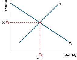
• Comparative Statics: Start with an initial equilibrium, change one variable, and compare the new equilibrium to the original.

• Application: In microeconomics, this involves the intersection of supply and demand; in macroeconomics, it involves the intersection of aggregate supply and aggregate demand.

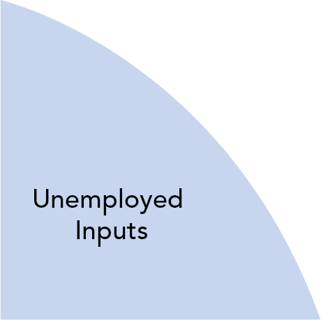
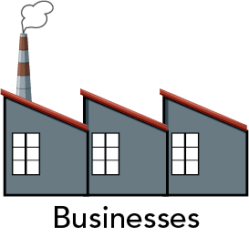
The Circular Flow Model

The circular flow model illustrates the movement of goods, services, and money in the economy, showing the interactions between households, businesses, and markets.

Aggregate Supply and Aggregate Demand Model

The AS/AD model explains how the economy achieves or misses targets such as potential GDP, full employment, and stable prices. Shocks to aggregate supply or demand can cause business cycles, unemployment, and inflation.

• Supply Shocks: Unexpected events that affect production costs or input availability.

• Demand Shocks: Changes in spending plans due to expectations, policy, or external factors.

Macroeconomic Performance Targets: Potential GDP and Long-Run Aggregate Supply

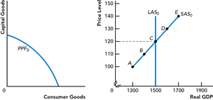
Potential GDP represents the maximum sustainable output of an economy when all resources are fully employed. The long-run aggregate supply (LAS) curve is vertical at potential GDP, indicating that output does not depend on the price level in the long run.

• Production Possibilities Frontier (PPF): Shows the maximum combinations of goods and services that can be produced with available resources.

• LAS Curve: Vertical at potential GDP; unaffected by price level changes.

Short-Run vs. Long-Run Aggregate Supply

The distinction between short-run and long-run in macroeconomics is based on price and wage flexibility:

• Short Run: Some input prices (especially wages) are fixed; output prices are flexible.

• Long Run: All prices and wages are flexible; the economy operates at potential GDP.

Short-Run Aggregate Supply (SAS)

Short-run aggregate supply reflects the quantity of real GDP that firms plan to produce at different price levels, holding input prices constant. The law of short-run aggregate supply states that as the price level rises, the quantity supplied increases.

• Movement Along SAS: Caused by changes in the price level.

• Shifts in SAS: Caused by changes in input prices or supply shocks.

Shifts in Aggregate Supply

Changes in the quantity or quality of inputs shift both the LAS and SAS curves in the same direction. Increases in inputs shift the curves rightward, while decreases shift them leftward.

• Input Price Changes: Affect only SAS, not LAS.

• Supply Shocks: Negative shocks (e.g., higher oil prices) shift SAS left; positive shocks (e.g., technological improvements) shift SAS right.

Part 2: Aggregate Demand

Aggregate Demand (AD)

Aggregate demand is the total quantity of real GDP that all sectors (households, businesses, government, and the rest of the world) plan to buy at different price levels. The law of aggregate demand states that as the price level rises, the quantity of real GDP demanded falls.

• Components of AD: Consumption (C), Investment (I), Government Spending (G), Net Exports (X – IM).

• Equation:

Determinants and Shocks to Aggregate Demand

Aggregate demand can shift due to changes in expectations, interest rates, government policy, foreign GDP, and exchange rates. These are called demand shocks.

• Negative Demand Shock: Shifts AD left (e.g., pessimistic expectations, higher interest rates).

• Positive Demand Shock: Shifts AD right (e.g., optimistic expectations, lower taxes).

Macroeconomic Equilibrium

Short-run equilibrium occurs where SAS and AD intersect. Long-run equilibrium is where SAS, AD, and LAS all intersect, meaning the economy is at potential GDP with full employment and stable prices.

• Steady Growth: Achieved through business investment that increases inputs, shifting LAS, SAS, and AD rightward over time.

Aggregate Supply and Demand Shocks

Types of Macroeconomic Shocks

• Negative Demand Shock: Causes recessionary gap (lower GDP, higher unemployment, lower prices).

• Positive Demand Shock: Causes inflationary gap (higher GDP, lower unemployment, higher prices).

• Negative Supply Shock: Causes stagflation (higher prices, lower GDP, higher unemployment).

• Positive Supply Shock: Increases GDP, lowers prices, maintains full employment.

Using the AS/AD Model for Economic Analysis

To analyze macroeconomic events, start from long-run equilibrium and use comparative statics to assess the impact of shocks. The AS/AD model helps predict changes in real GDP, unemployment, and inflation, and guides policy debates between 'hands-off' (market self-correction) and 'hands-on' (policy intervention) approaches.