Aggregate Supply (AS) Curve

Definition and Characteristics

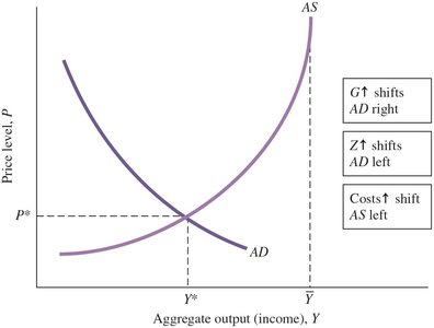
The aggregate supply (AS) curve represents the total supply of all goods and services in an economy at various price levels. It is a "price/output response" curve, tracing the price and output decisions of all firms under different levels of aggregate demand.

• Aggregate supply: The total supply of goods and services produced within an economy.

• AS curve: Shows the relationship between aggregate output and the overall price level.

• In the short run, the AS curve is upward sloping, reflecting that higher prices can lead to increased output.

• At low output levels, the curve is flat; as the economy nears capacity, it becomes nearly vertical.

Why the AS Curve is Upward Sloping

Wages, a major component of costs, tend to lag behind price changes. This lag causes the short-run AS curve to slope upward, as firms respond to higher prices by increasing output.

• At low output, small price increases yield large output responses.

• At capacity, further increases in demand only raise prices, not output.

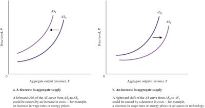
Shifts of the Short-Run AS Curve

The AS curve can shift due to changes in production costs, known as cost shocks or supply shocks. Examples include changes in energy prices or technological advances.

• A leftward shift indicates a decrease in aggregate supply (higher costs).

• A rightward shift indicates an increase in aggregate supply (lower costs).

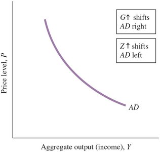
Aggregate Demand (AD) Curve

Derivation and Properties

The aggregate demand (AD) curve is derived from the goods market and the behavior of the Federal Reserve (Fed). It shows the relationship between the aggregate output and the price level, with a downward slope.

• AD is not the sum of individual market demand curves.

• When the price level rises, the Fed raises the interest rate, reducing investment and output.

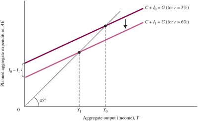
Planned Aggregate Expenditure and the Interest Rate

Planned aggregate expenditure (AE) is affected by the interest rate. As the interest rate rises, planned investment falls, reducing AE and equilibrium output.

• Formula:

• Higher interest rates () discourage investment (), lowering AE and output ().

• Lower interest rates encourage investment, raising AE and output.

The IS Curve

The IS curve shows the negative relationship between aggregate output and the interest rate in the goods market. Each point on the IS curve represents equilibrium for a given interest rate.

• Increase in government spending () shifts the IS curve right, increasing output.

The Behavior of the Fed

Fed Rule and Policy Decisions

The Fed uses output () and inflation () as inputs for its interest rate decisions. The Fed rule is an equation showing how the Fed sets the interest rate based on economic conditions:

• Fed rule:

• represents other unpredictable economic factors.

• The Fed aims to balance maximum employment and stable prices.

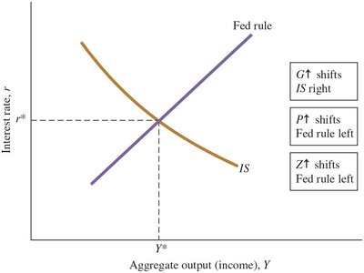
Equilibrium in the Goods and Money Markets

Intersection of IS and Fed Rule

The equilibrium values of output and the interest rate are determined by the intersection of the IS curve and the Fed rule. Changes in government spending, price level, or other factors shift these curves.

• Increase in shifts IS right.

• Increase in or shifts Fed rule left.

Deriving the AD Curve

The AD curve is derived from the equilibrium in the goods and money markets. When the price level increases, the Fed raises the interest rate, reducing investment and output, resulting in a downward-sloping AD curve.

Final Equilibrium: Output and Price Level

Intersection of AS and AD Curves

Aggregate output and the aggregate price level are determined by the intersection of the AS and AD curves. This intersection reflects the combined decisions of households, firms, and the government.

Other Reasons for a Downward-Sloping AD Curve

Real Wealth Effect

Besides the Fed's response to price changes, the real wealth effect also contributes to the downward slope of the AD curve. When the price level rises, real wealth falls, reducing consumption and aggregate demand.

• Real wealth effect: Change in consumption due to changes in real wealth from price level changes.

The Long-Run Aggregate Supply Curve

Shape and Adjustment

The long-run AS curve is vertical, reflecting the economy's potential output. In the long run, wages and prices fully adjust, and output returns to potential GDP.

• Short-run shifts in AD can temporarily increase output and price level.

• Long-run wage adjustments shift AS back, restoring output to potential GDP.

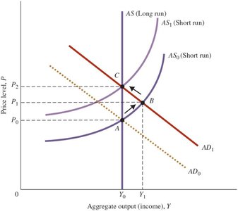
Potential GDP

Definition and Implications

Potential output or potential GDP is the level of aggregate output that can be sustained in the long run without inflation. The vertical portion of the short-run AS curve represents the physical limits of production.

• Economists debate how to determine if the economy is at or above potential output.

• Some believe output rises when wages fall with high unemployment.

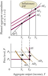
Keynesian Aggregate Supply Curve and Inflationary Gap

Short-Run and Inflationary Gap

The "Keynesian" AS curve illustrates how shifts in planned aggregate expenditure and AD affect output and price level. If AE and AD exceed potential output, an inflationary gap arises, causing the price level to rise.

• Equilibrium output rises with increased AE and AD, but price level remains constant until capacity is reached.

• Beyond capacity, price level increases, creating an inflationary gap.

Review Terms and Concepts

• Aggregate supply

• Aggregate supply (AS) curve

• Cost shock, or supply shock

• Fed rule

• IS curve

• Potential output, or potential GDP

• Real wealth effect

Key Equations