Consumption-Savings Decision

Introduction

The consumption-savings decision is a fundamental topic in macroeconomics, focusing on how households allocate their income between current consumption and saving for future consumption. This decision is influenced by factors such as current and future income, real interest rates, and fiscal policy. Understanding these choices helps explain aggregate consumption and saving behavior in the economy.

Key Definitions and Concepts

Desired Consumption and Saving

- Desired consumption (Cd): The aggregate quantity of goods and services households wish to consume, given their income and other factors. - Desired saving (Sd): The level of national saving when aggregate consumption equals desired consumption. - Private saving (Sdp): The portion of saving done by households. - Closed economy assumption: No net factor payments (NFP = 0), so saving is simply the difference between income and consumption plus government spending.

Consumption-Smoothing Motive

Households generally prefer a stable pattern of consumption over time, known as the consumption-smoothing motive. - Temporary income increases are often saved and spread over future periods. - Permanent income increases raise consumption in all periods.

Two-Period Model of Consumption and Saving

Model Structure

The two-period model divides time into today (period 1) and the future (period 2). Households face perfect capital markets, meaning no borrowing constraints and equal interest rates for borrowing and saving.

Indifference Curves

Indifference curves represent combinations of current (C1) and future (C2) consumption that yield the same utility level. - The curve is negatively sloped: increasing C1 requires reducing C2 to maintain the same utility. - The slope, , measures the trade-off between current and future consumption.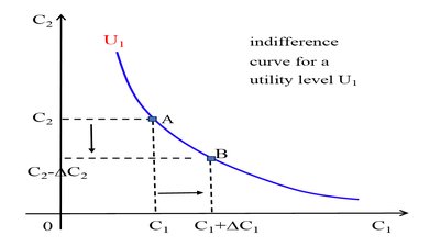

Indifference Curves at Different Utility Levels

Higher indifference curves represent higher utility levels. Moving to a higher curve means greater overall satisfaction.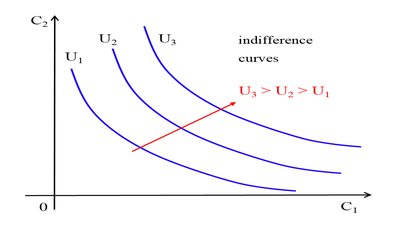

Budget Constraints

Budget Constraints in Two Periods

- Today’s budget constraint: where V is initial financial assets. - Future consumption: - Intertemporal budget constraint: Substitute Sp from today’s constraint into the future constraint: Divide by and rearrange: where W is total wealth.

Graphical Representation

The intertemporal budget constraint is a straight line with slope , showing the trade-off between current and future consumption.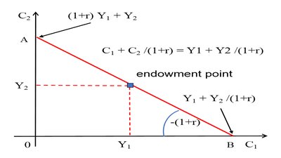

Optimal Consumption Choices

Saver’s Optimal Choice

A saver chooses a consumption profile where current consumption is less than current income, resulting in positive saving. The optimal point is where the highest indifference curve is tangent to the budget constraint.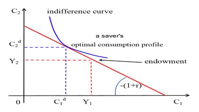

Borrower’s Optimal Choice

A borrower chooses a consumption profile where current consumption exceeds current income, resulting in negative saving (borrowing).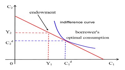

Effects of Changes in Income

Increase in Current Income (Y1)

An increase in current income shifts the budget constraint upward in a parallel fashion, allowing for higher consumption in both periods.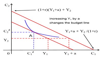

Saver’s Response to Higher Y1

The saver’s optimal consumption profile shifts, increasing both current and future consumption.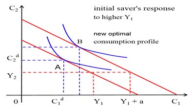

Borrower’s Response to Higher Y1

The borrower’s optimal consumption profile also shifts, increasing both current and future consumption.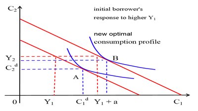

Marginal Propensity to Consume (MPC)

Definition and Implications

- Marginal propensity to consume (MPC): The fraction of additional current income that is consumed in the current period. - Typically, MPC < 1, meaning part of the income increase is saved. - To measure MPC accurately, expected future income must be held constant.

Effects of Changes in Future Income

Increase in Future Income (Y2)

An increase in future income shifts the budget constraint, allowing for higher current consumption and reducing private saving.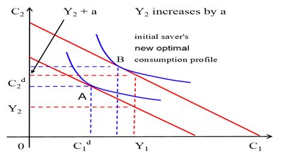

Effects of Changes in Real Interest Rate (r)

Budget Constraint Rotation

An increase in the real interest rate changes the slope of the budget constraint, making future consumption relatively cheaper.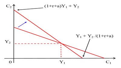

Substitution and Income Effects

- Substitution effect: Higher r makes future consumption cheaper, so consumers substitute away from current consumption to future consumption. - Income effect: Depends on whether the consumer is a saver or borrower: - If Sp > 0 (saver): Higher r increases future income, leading to higher consumption in both periods. - If Sp < 0 (borrower): Higher r increases debt burden, leading to lower consumption in both periods.

Saver’s Response: Substitution Effect Dominates

When the substitution effect dominates, the saver reduces current consumption and increases saving.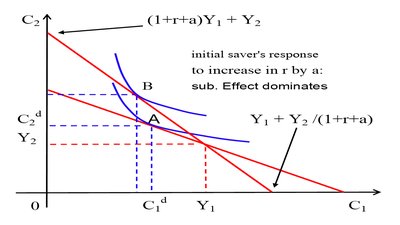

Saver’s Response: Income Effect Dominates

When the income effect dominates, the saver increases current consumption and reduces saving.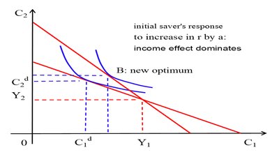

Borrower’s Response to Higher r

The borrower reduces current consumption and increases saving (reduces borrowing) in response to a higher interest rate.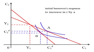

Summary Table: Effects of Interest Rate Changes

Comparison of Saver and Borrower Responses

Empirical Evidence

Empirical studies suggest that an increase in the real interest rate generally reduces current consumption and increases saving, but the effect is not very strong.

Conclusion

The consumption-savings decision is central to understanding household behavior in macroeconomics. Changes in income and interest rates affect both consumption and saving, with the effects depending on whether households are savers or borrowers and the relative strength of substitution and income effects. Key formulas: Additional info: The notes above expand on the original slides by providing definitions, context, and examples for each concept, ensuring completeness and academic clarity.