The Three Macro Time Frames

Short Run, Adjustment Process, and Long Run

The macroeconomy is analyzed across three distinct time frames: the short run, the adjustment process, and the long run. Each period is characterized by different assumptions about factor prices, technology, and factor supplies.

• Short Run: Real GDP is determined by the Aggregate Demand-Aggregate Supply (AD-AS) model. Factor prices (such as wages and commodity prices) are exogenous, and both technology and factor supplies are constant, so potential output (Y*) is fixed.

• Adjustment Process: Factor prices become endogenous and respond to output gaps, allowing real GDP to return to potential. Technology and factor supplies remain constant.

• Long Run: Factor prices are fully adjusted, and technology and factor supplies change over time, causing potential output (Y*) to shift.

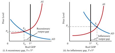
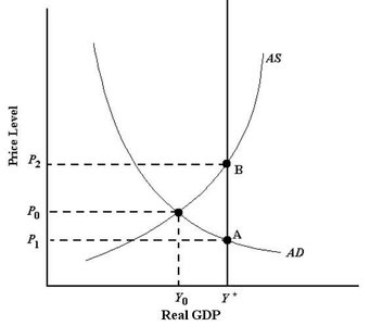
Potential GDP is the total output produced when all factors of production are fully employed. Output gaps (recessionary or inflationary) occur when actual GDP deviates from potential GDP.

Closing Output Gaps

Recessionary and Inflationary Gaps

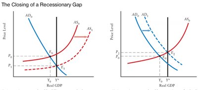
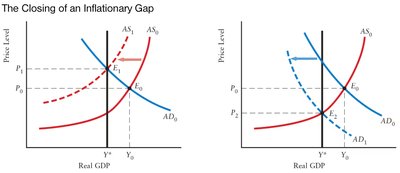
Output gaps induce changes in factor prices, which in turn affect production costs and shift the aggregate supply curve. The adjustment process is asymmetric: recessionary gaps lead to slow wage decreases, while inflationary gaps cause rapid wage increases.

• Recessionary Gap: Excess supply of labor and other factors leads to falling wages and unit costs, shifting AS right and returning GDP to potential.

• Inflationary Gap: Excess demand for labor and other factors causes rising wages and unit costs, shifting AS left and closing the gap.

• Sticky Wages: Wages and other factor prices may be slow to adjust downward due to contracts and benefits, prolonging recessionary gaps.

• At Y = Y*: Employment is at full employment, and the unemployment rate equals the natural rate (NAIRU), with no cyclical unemployment.

Shocks and the Adjustment Process

AD and AS Shocks

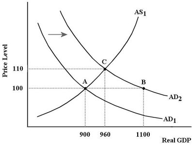
Aggregate demand (AD) and aggregate supply (AS) shocks temporarily move real GDP away from potential output. The adjustment process returns GDP to potential, with factor prices adjusting accordingly.

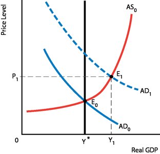
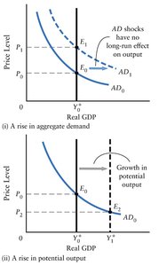
• Positive AD Shock: Increases real GDP and price level in the short run, but does not affect GDP in the long run.

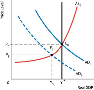
• Negative AD Shock: Decreases real GDP and price level in the short run, but long-run GDP remains unchanged.

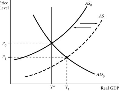
• Positive AS Shock: Decreases costs, increases real GDP, and lowers price level in the short run. AS shifts left during adjustment, returning GDP to potential.

Long-Run Equilibrium

AD-AS Equilibrium and Determinants

In the long run, factor prices are fully adjusted and there are no output gaps. The intersection of AD and the long-run aggregate supply (LRAS) curve determines the price level, while real GDP is set by potential output (Y*).

• LRAS: The long-run aggregate supply curve is a vertical line at Y*, reflecting the classical view that real GDP is determined by resources and productivity.

• Positive AD Shock: Shifts AD right, raising the price level but leaving real GDP unchanged in the long run.

• Growth in Potential GDP: LRAS shifts right if resources or productivity increase, raising potential output.

Fiscal Stabilization Policy

Discretionary Fiscal Policy and Automatic Stabilizers

Fiscal policy can be used to stabilize the economy in response to AD and AS shocks. Governments may choose to wait for the adjustment process or intervene with discretionary fiscal policy.

• Discretionary Fiscal Policy: Deliberate changes in government spending, taxes, or transfer payments to influence real GDP. Used to close recessionary or inflationary gaps.

• Time Lags: Recognition lag (identifying recession), decision lag (policy changes), and execution lag (implementing policy) limit the effectiveness of discretionary fiscal policy.

• Automatic Fiscal Stabilizers: Tax and transfer systems automatically reduce GDP fluctuations. For example, higher taxes and lower transfers during booms dampen the impact of shocks.

• Simple Multiplier: The effect of fiscal policy depends on the multiplier, calculated as , where .

• Long-Term Impact: Fiscal policy rarely affects potential GDP unless it increases productivity (e.g., infrastructure investment).

Exercises and Applications

Identifying Macro Time Frames and Output Gaps

Students should be able to match macroeconomic concepts to their definitions and fill in model assumptions for each time frame. Output gaps can be identified using real GDP and wage change data.

Example: Economies D and E are experiencing inflationary gaps and rising wages.

Fiscal Policy Calculations

To close a recessionary gap, the required change in government spending can be calculated using the multiplier:

• Formula:

• Example: If the output gap is 60 and the multiplier is 1.2, then

Automatic Stabilizers and Multiplier Effects

Economies with higher net tax rates have smaller multipliers and are less susceptible to fluctuations from autonomous expenditure shocks.

Economy B's lower tax rate produces larger fluctuations in real GDP.

Limitations of Fiscal Policy

• Decision lags and expenditure lags

• Risk of overshooting

• Temporary vs. permanent policy perceptions