Q1. What happens to consumption spending when income increases, and how does a change in expected future income or household wealth affect the consumption function?

Background

Topic: Consumption Function in Macroeconomics

This question tests your understanding of how changes in income and other factors affect consumption spending and the position of the consumption function in the aggregate expenditure model.

Key Terms and Formulas:

• Consumption Function: Shows the relationship between consumption spending and real national income (or real GDP).

• Marginal Propensity to Consume (MPC): The fraction of additional income that is spent on consumption.

• Autonomous Consumption: Consumption that occurs even when income is zero, often affected by household wealth and expected future income.

Step-by-Step Guidance

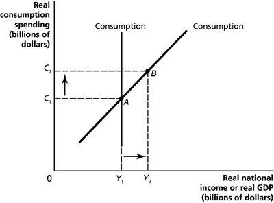
1. Examine the graph of the consumption function. Notice that as real national income (Y) increases from to , real consumption spending also increases from to along the same consumption function.

2. Understand that this movement from point A to point B represents a change in consumption due to a change in income, holding other factors constant. This is a movement along the consumption function.

3. Recognize that if expected future income or household wealth increases, the entire consumption function shifts upward. This means, for any given level of income, consumption spending will be higher.

4. Identify the difference between a movement along the consumption function (caused by a change in income) and a shift of the consumption function (caused by changes in wealth or expectations).

Try solving on your own before revealing the answer!

Q2. What does the 45°-line diagram illustrate in the aggregate expenditure model, and how is macroeconomic equilibrium determined?

Background

Topic: 45°-Line Diagram and Macroeconomic Equilibrium

This question tests your ability to interpret the 45°-line diagram and understand how equilibrium real GDP is determined in the aggregate expenditure model.

Key Terms and Formulas:

• Aggregate Expenditure (AE): The total spending in the economy (C + I + G + NX).

• Macroeconomic Equilibrium: Occurs where planned aggregate expenditure equals real GDP.

• 45° Line: Represents all points where AE = Y (real GDP).

Step-by-Step Guidance

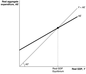
1. Look at the 45°-line diagram. The 45° line shows all points where aggregate expenditure equals real GDP.

2. The aggregate expenditure line (AE) shows the relationship between planned spending and real GDP.

3. Macroeconomic equilibrium is found at the intersection of the AE line and the 45° line. At this point, planned spending equals actual output.

4. If AE is above the 45° line, inventories will decrease, and firms will increase production. If AE is below the 45° line, inventories will increase, and firms will decrease production.

Try solving on your own before revealing the answer!

Q3. How do unintended changes in inventories indicate whether the economy is above or below equilibrium in the aggregate expenditure model?

Background

Topic: Inventories and Macroeconomic Equilibrium

This question tests your understanding of how inventory changes signal whether the economy is at, above, or below equilibrium in the aggregate expenditure model.

Key Terms and Formulas:

• Unintended Change in Inventories: The difference between actual output (real GDP) and planned aggregate expenditure.

• Equilibrium: Occurs when there is no unintended change in inventories (AE = Y).

• Formula:

Step-by-Step Guidance

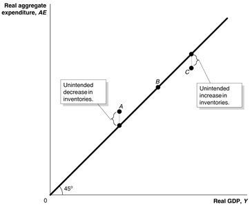
1. Examine the diagram showing points A, B, and C relative to the 45° line and the AE line.

2. At point A, planned aggregate expenditure is greater than real GDP, leading to an unintended decrease in inventories.

3. At point C, planned aggregate expenditure is less than real GDP, leading to an unintended increase in inventories.

4. At point B, planned aggregate expenditure equals real GDP, so there is no unintended change in inventories—this is equilibrium.

Try solving on your own before revealing the answer!

Q4. Why is the net exports line downward sloping in the aggregate expenditure model?

Background

Topic: Net Exports and Aggregate Expenditure

This question tests your understanding of how net exports are affected by changes in real GDP and why the net exports line slopes downward in the aggregate expenditure model.

Key Terms and Formulas:

• Net Exports (NX): The value of exports minus the value of imports.

• Real GDP: The total value of goods and services produced in the economy, adjusted for inflation.

Step-by-Step Guidance

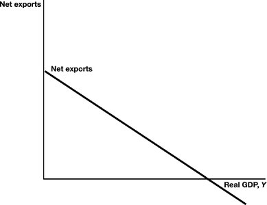
1. Understand that net exports are affected by changes in real GDP. As real GDP increases, imports tend to rise because consumers and firms buy more foreign goods.

2. Exports are not directly affected by domestic real GDP, but imports increase, causing net exports to decline.

3. This relationship is shown as a downward-sloping line in the aggregate expenditure model.

4. The slope reflects the negative relationship between real GDP and net exports.

Try solving on your own before revealing the answer!

Q5. How does a decrease in government purchases affect equilibrium real GDP in the aggregate expenditure model?

Background

Topic: Government Purchases and the Multiplier Effect

This question tests your understanding of how changes in government spending impact aggregate expenditure and equilibrium real GDP, including the multiplier effect.

Key Terms and Formulas:

• Aggregate Expenditure (AE): Total spending in the economy.

• Multiplier Effect: The process by which a change in autonomous expenditure leads to a larger change in real GDP.

• Multiplier Formula:

Step-by-Step Guidance

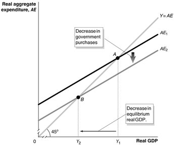
1. Observe the diagram showing a decrease in government purchases, which shifts the AE line downward from AE1 to AE2.

2. This shift causes equilibrium real GDP to decrease from to .

3. The decrease in real GDP is larger than the initial decrease in government purchases due to the multiplier effect.

4. Calculate the change in equilibrium real GDP using the multiplier formula and the change in government purchases.

Try solving on your own before revealing the answer!

Q6. What happens to equilibrium real GDP when autonomous expenditure increases, and how is this shown in the aggregate expenditure model?

Background

Topic: Autonomous Expenditure and the Multiplier Effect

This question tests your understanding of how increases in autonomous expenditure affect equilibrium real GDP, using the aggregate expenditure model and the multiplier effect.

Key Terms and Formulas:

• Autonomous Expenditure: Spending that does not depend on the level of income or GDP.

• Multiplier Effect:

• Equilibrium Real GDP: The level of GDP where AE = Y.

Step-by-Step Guidance

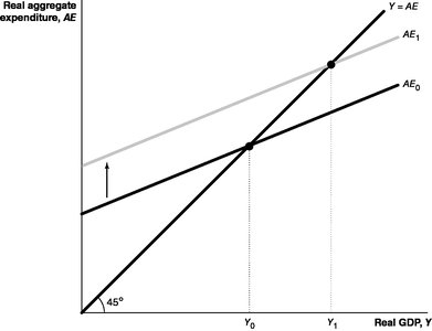
1. Examine the diagram showing the AE line shifting upward from AE0 to AE1 due to an increase in autonomous expenditure.

2. This shift causes equilibrium real GDP to increase from to .

3. The increase in real GDP is greater than the initial increase in autonomous expenditure because of the multiplier effect.

4. Calculate the change in equilibrium real GDP using the multiplier formula and the change in autonomous expenditure.

Try solving on your own before revealing the answer!