Chapter 11: The Determination of Aggregate Output, the Price Level, and the Interest Rate

Introduction

This chapter integrates the concepts of aggregate output, the price level, and the interest rate to explain how equilibrium is determined in the macroeconomy. It provides the foundation for understanding how policymakers manage economic fluctuations and address issues such as inflation, unemployment, and economic growth.

Aggregate Supply (AS) Curve

Definition and Characteristics

• Aggregate supply (AS): The total supply of all goods and services produced within an economy.

• AS curve: A graphical representation showing the relationship between the aggregate quantity of output supplied and the overall price level.

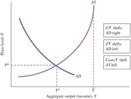
• The AS curve is also known as the "price/output response" curve, reflecting how firms adjust output and prices in response to changes in aggregate demand.

Short-Run Aggregate Supply (SRAS)

• In the short run, the AS curve is upward sloping.

• At low levels of output, the curve is relatively flat, indicating that small price increases can lead to large increases in output.

• As the economy approaches its productive capacity, the curve becomes steeper and eventually vertical, reflecting physical limits to production.

• Reason for upward slope: Wages, a major component of costs, tend to adjust more slowly than prices, causing firms to increase output as prices rise.

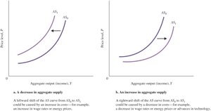
Shifts in the Short-Run AS Curve

• The vertical portion of the SRAS curve represents the economy's maximum output, determined by available resources.

• Cost shock (supply shock): Any event that changes production costs (e.g., oil price changes, technological advances) can shift the SRAS curve.

Aggregate Demand (AD) Curve

Derivation and Slope

• The AD curve is derived from the goods market (IS curve) and the monetary sector (Fed rule).

• It shows the relationship between the aggregate price level and the quantity of output demanded.

• The AD curve is downward sloping because higher price levels lead the central bank (the Fed) to raise interest rates, which reduces investment and, consequently, aggregate output.

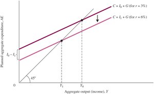
Planned Aggregate Expenditure and the Interest Rate

• As the interest rate (r) rises, planned investment (I) falls, reducing total planned spending and equilibrium output.

• A decrease in aggregate expenditure (AE) lowers equilibrium output by a multiple of the initial decrease in investment.

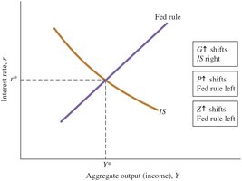
The IS Curve

• The IS curve shows the negative relationship between aggregate output and the interest rate in the goods market.

• Any point on the IS curve represents equilibrium in the goods market for a given interest rate.

• An increase in government spending shifts the IS curve to the right, increasing output at any given interest rate.

The Fed Rule

• The Fed sets the interest rate based on the state of the economy, particularly output (Y) and inflation (P).

• The Fed rule can be expressed as an equation relating the interest rate to output, inflation, and other factors (Z).

• When output or inflation rises, the Fed typically raises the interest rate to maintain stability.

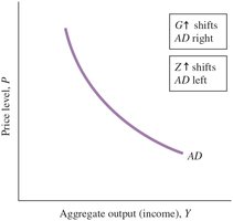
Deriving the AD Curve

• The AD curve is not a simple sum of market demand curves; it reflects the equilibrium output for each price level, considering the Fed's response to inflation.

• When the price level rises, the Fed raises the interest rate, reducing investment and output, which creates the downward slope of the AD curve.

The Final Equilibrium

Intersection of AS and AD

• The equilibrium levels of aggregate output and the price level are determined by the intersection of the AS and AD curves.

• This intersection reflects the combined decisions of households, firms, and the government.

Other Reasons for a Downward-Sloping AD Curve

• Besides the interest rate effect, the real wealth effect also contributes to the downward slope of the AD curve.

• Real wealth effect: When the price level falls, the real value of wealth increases, leading to higher consumption and aggregate demand.

The Long-Run Aggregate Supply (LRAS) Curve

Shape and Adjustment

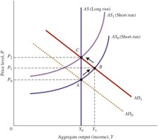
• In the long run, the AS curve is vertical at the level of potential output (potential GDP).

• When the AD curve shifts, the price level may rise in the short run, but wages and other input prices adjust over time, returning output to its long-run potential.

Potential GDP

• Potential output (potential GDP): The maximum level of aggregate output that can be sustained in the long run without causing inflation.

• The vertical portion of the SRAS curve reflects the economy's physical production limits.

• Economists debate how to determine whether the economy is operating at or above potential output.

The Simple "Keynesian" Aggregate Supply Curve

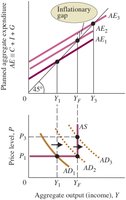
• In the Keynesian model, increases in planned aggregate expenditure shift the AD curve, raising output without affecting the price level until the economy reaches full capacity.

• If aggregate expenditure and demand exceed potential output, an inflationary gap arises, causing the price level to rise.

Key Terms and Concepts

• Aggregate supply (AS)

• Aggregate supply (AS) curve

• Cost shock (supply shock)

• Fed rule

• IS curve

• Potential output (potential GDP)

• Real wealth effect

Key Equations

• IS Curve:

• Fed Rule (example):

• Aggregate Demand:

Additional info: The IS curve equation shows the relationship between output and the interest rate, while the Fed rule describes how the central bank sets the interest rate in response to economic conditions. The AD equation summarizes total spending in the economy.