The Phillips Curve

Introduction to the Phillips Curve

The Phillips Curve describes the empirical relationship between the rate of inflation (πt) and the unemployment rate (ut). It suggests a tradeoff: lower unemployment is associated with higher inflation, and vice versa. This relationship has important implications for macroeconomic policy, especially for central banks targeting inflation and employment.

• Negative Relationship: Historically, periods of low unemployment have coincided with higher inflation rates.

• Policy Implication: Efforts to reduce inflation may require tolerating higher unemployment, at least in the short run.

Historical Evidence: The U.S. Experience

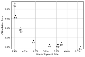
• 1960s: Low and stable inflation, strong negative correlation between inflation and unemployment.

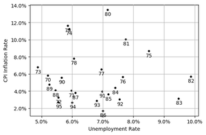
• 1970–1995: Oil price shocks led to higher inflation and shifting expectations, weakening the simple Phillips Curve relationship.

• 1996–2019: The Federal Reserve anchored inflation expectations around 2%, stabilizing the relationship.

Deriving the Phillips Curve from the Labor Market

The Phillips Curve can be derived from wage-setting and price-setting behavior in the labor market. The key equations are:

• Wage-setting: W = PeF(u, z)

• Price-setting: P = (1 + m)W

Where:

• W: Nominal wage

• P: Price level

• Pe: Expected price level

• u: Unemployment rate

• z: Other factors affecting wage bargaining (e.g., labor laws, unions)

• m: Markup of prices over costs

From Price Level to Inflation

Inflation is defined as the percentage change in the price level:

By substituting and manipulating the wage and price equations, and using a log-linear approximation, we obtain a linearized Phillips Curve:

Where:

• \(\pi_t\): Actual inflation

• \(\pi_t^e\): Expected inflation

• \(\alpha\): Sensitivity of inflation to unemployment

• \(m\): Markup

• \(z\): Other factors affecting wage bargaining

Properties of the Phillips Curve

• Expected Inflation: Higher expected inflation leads to higher actual inflation, as workers demand higher wages and firms raise prices accordingly.

• Markup (m): An increase in the markup raises inflation at any unemployment rate.

• Worker Bargaining Power (z): Policies or factors that increase worker bargaining power also increase inflation.

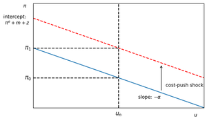
Graphical Representation and Cost-Push Shocks

The Phillips Curve can shift due to changes in markup or other cost factors ("cost-push" shocks). For example, a rise in oil prices increases production costs, shifting the curve upward and leading to higher inflation at every unemployment rate.

Testing the Phillips Curve

The Phillips Curve is testable using regression analysis:

Key variables:

• Current inflation (\(\pi_t\))

• Expected inflation (\(\pi_t^e\))

• Unemployment rate (\(u_t\))

• Markup (m)

• Other factors (z)

Measuring Expected Inflation

• Survey Data: Directly ask households or professionals for their inflation expectations (e.g., Philadelphia Fed Survey of Professional Forecasters).

• Market Data: Use the difference between nominal and inflation-indexed bond yields (e.g., TIPS).

Empirical Evidence: U.S. Data

The 1960s: Anchored Expectations

During the 1960s, inflation was low and stable, and expectations were anchored. The Phillips Curve predicted a strong negative relationship between inflation and unemployment.

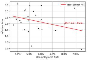
1970–1995: Unanchored Expectations and Oil Shocks

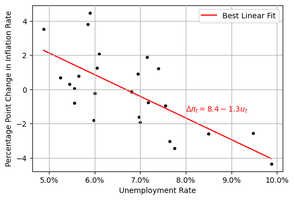
Large oil price shocks led to higher inflation and unanchored expectations. The relationship between inflation and unemployment became less clear, but the Phillips Curve still predicted a negative relationship between the change in inflation and unemployment:

1996–2019: Anchored Expectations and Inflation Targeting

With the Federal Reserve targeting 2% inflation, expectations became anchored again, and the Phillips Curve relationship stabilized.

Long-Run and Medium-Run Equilibrium

In the medium run, the Phillips Curve can be expressed relative to the natural rate of unemployment (un):

Where:

• \(u_n\): Natural rate of unemployment, determined by markup and bargaining power:

Interpretation:

• If \(u_t = u_n\), inflation is stable at the target.

• If \(u_t > u_n\), inflation falls below the target.

• If \(u_t < u_n\), inflation rises above the target.

Summary Table: Phillips Curve Equations

Conclusion

The Phillips Curve remains a central concept in macroeconomics, linking inflation, unemployment, and expectations. Its empirical relevance depends on how expectations are formed and on the presence of shocks such as changes in oil prices or policy regimes. Understanding the Phillips Curve helps policymakers anticipate the effects of monetary and fiscal interventions on inflation and employment.