Chapter 6: The Simple Short-Run Macroeconomic Model

Introduction to the Keynesian Short-Run Model

The Keynesian short-run macroeconomic model posits that aggregate demand determines output in the short term. In a closed economy without a government sector, understanding the drivers of aggregate expenditures is crucial for analyzing output and employment.

Aggregate Expenditures in a Closed Economy

Aggregate Expenditures (AE) represent the total planned spending on a country's output. In a closed economy with no government sector, the formula simplifies to:

• AE = C + I

• C: Consumption Expenditures

• I: Investment Expenditures

Determinants of Household Consumption (C)

Household consumption is influenced by several factors:

• Personal Disposable Income (YD or DI): The income available to households after taxes.

• Households’ Wealth (W): Higher wealth increases consumption.

• Consumer Confidence (HEx): Positive expectations boost spending.

• Real Interest Rates (r): Lower rates encourage consumption.

• Household Debt (D): High debt can reduce consumption.

• Taxes (T): Affect disposable income.

Relationship Between Consumption, Savings, and Disposable Income

Disposable income is allocated between consumption and savings:

• YD = C + S

• Average Propensity to Consume (APC): Fraction of income spent:

• Average Propensity to Save (APS): Fraction of income saved:

• APC + APS = 1

• Marginal Propensity to Consume (MPC): Fraction of additional income spent:

• Marginal Propensity to Save (MPS): Fraction of additional income saved:

• MPC + MPS = 1

Example Calculation

Suppose income increases from $154,897 to $161,580 and consumption from $128,600 to $132,745:

The Consumption Function

The consumption function describes the relationship between consumption and disposable income:

• C0: Autonomous consumption (spending not from current income)

• mpc: Marginal propensity to consume (slope of the consumption curve)

Example:

Shifts in the Consumption Curve

Factors other than disposable income can shift the consumption curve:

• Households’ Wealth: Increase shifts curve up.

• Consumer Confidence: Increase shifts curve up.

• Real Interest Rates: Decrease shifts curve up.

• Household Debt: Decrease shifts curve up.

These factors affect autonomous consumption ().

Personal Saving Equation

From , the saving function is:

• Example: If , then

Break-Even Disposable Income

Break-even disposable income () is where households spend exactly their disposable income:

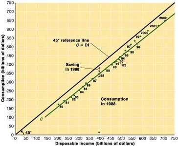
The 45° Line and Consumption

The 45° line on a graph of consumption vs. disposable income represents points where . It is used to identify break-even points and analyze saving behavior.

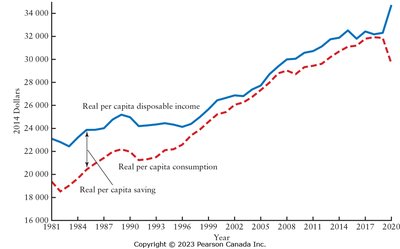
Trends in Consumption, Income, and Saving

Over time, real per capita disposable income and consumption generally rise, with saving fluctuating based on economic conditions.

Determinants of Gross Business Investment (Ig)

Business investment expenditures are influenced by:

• Interest Rates: Lower rates increase investment.

• Expected Rate of Profit: Higher expected profits increase investment.

• Government Policy: Higher taxes/regulation decrease investment.

• Technological Change: Increases investment.

• Capacity Utilization: Higher utilization increases investment.

• Business Confidence: Positive expectations increase investment.

Investment Demand Curve and Schedule

The investment demand curve shows the inverse relationship between investment and interest rates. The investment schedule relates investment to national income, but in the short-run model, investment is autonomous (does not depend on current income).

Aggregate Expenditures Equation

The aggregate expenditures equation is:

• A0: Autonomous expenditures (vertical intercept)

• z: Marginal propensity to spend (slope, equals mpc in this model)

Example: If and , then

Macroeconomic Equilibrium

Equilibrium occurs when:

• Unplanned Inventory Change (UIC) is zero:

• Total Injections = Total Leakages:

Equilibrium output () can be found by:

1. Solving the model algebraically

2. Using the formula:

3. Reading from a table

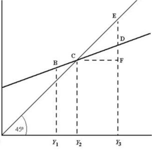
Adjustment to Equilibrium

If output exceeds equilibrium (), inventories accumulate and firms reduce output. If output is below equilibrium (), inventories fall and firms increase output.

Changing Equilibrium Output

Equilibrium output can be changed by:

• Changing the marginal propensity to spend ()

• Changing autonomous expenditures ()

The Multiplier Effect

A change in autonomous expenditures leads to a multiplied change in output. The expenditures multiplier is calculated as:

• Formula 1:

• Formula 2:

Example: If , then

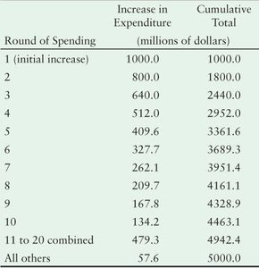
Multiplier Process Table

The multiplier process shows how an initial increase in spending leads to successive rounds of increased expenditure, each smaller than the last, until the total effect is realized.

Summary

The simple short-run macroeconomic model demonstrates how aggregate demand determines output in a closed economy without government. Key concepts include the consumption function, saving function, investment determinants, aggregate expenditures, equilibrium, and the multiplier effect. Understanding these relationships is fundamental for analyzing macroeconomic fluctuations and policy impacts.