Consumers and Incentives

Introduction

This chapter explores the fundamental decision-making process of consumers in microeconomics, focusing on how preferences, prices, and budgets interact to shape demand, consumer surplus, and elasticity. Understanding these concepts is essential for analyzing market behavior and predicting responses to changes in economic variables.

Key Ideas

• The buyer’s problem consists of three parts: preferences (what you like), prices, and your budget.

• Optimizing buyers make decisions at the margin, weighing additional benefits against additional costs.

• Individual demand curves reflect both ability and willingness to pay for goods and services.

• Consumer surplus is the difference between what a buyer is willing to pay and what they actually pay.

• Elasticity measures how responsive one variable is to changes in another.

The Buyer’s Problem

Three Components of the Buyer’s Problem

Consumers face three main questions when making purchasing decisions:

• What do you like? – Preferences and tastes determine the value placed on goods.

• How much does it cost? – Prices are assumed to be fixed and non-negotiable; consumers can buy as much as they want without affecting price.

• How much money do you have? – The budget set represents all possible combinations of goods a consumer can afford, given their income and prices.

Tastes and Preferences

Consumers aim to maximize their satisfaction (utility) given their preferences. Purchases signal individual tastes and priorities.

• Utility maximization – Consumers seek the greatest benefit for their money.

• Revealed preferences – Actual purchases reflect underlying tastes.

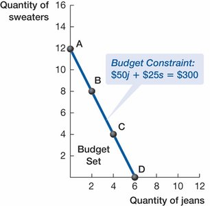
Budget Set and Budget Constraint

The budget set is the collection of all affordable bundles of goods. The budget constraint is the boundary of this set, defined by the consumer’s income and the prices of goods.

• No saving or borrowing – Only current income is used for purchases.

• Whole units – Purchases are made in whole numbers.

Budget Constraint Equation:

Opportunity Cost

Opportunity cost is the value of the next best alternative foregone when making a choice. In the context of the budget constraint, it is calculated as:

• Opportunity cost of jeans: Loss in sweaters / Gain in jeans

• Opportunity cost of sweaters: Loss in jeans / Gain in sweaters

Bundles on the Budget Constraint

Different combinations of goods (bundles) lie on the budget constraint, each representing a trade-off between goods.

Optimization and Marginal Analysis

Marginal Benefit per Dollar Spent

Consumers optimize by equating the marginal benefit per dollar spent across all goods:

• MB = Marginal Benefit

• P = Price

This condition ensures that the last dollar spent on each good yields the same additional benefit.

Budget Constraint Shifts and Pivots

Effects of Price and Income Changes

• Price Increase – Causes an inward pivot of the budget constraint, reducing affordable combinations.

• Price Decrease – Causes an outward pivot, increasing affordable combinations.

• Income Increase – Shifts the budget constraint outward, allowing more of both goods to be purchased.

From the Buyer’s Problem to the Demand Curve

Deriving the Demand Curve

The demand curve shows the relationship between price and quantity demanded. It is derived from the buyer’s optimization process.

• Negative slope – As price decreases, quantity demanded increases.

• Individual demand – Reflects both ability and willingness to pay.

Consumer Surplus

Definition and Calculation

Consumer surplus is the net benefit consumers receive from purchasing goods at market prices lower than their maximum willingness to pay.

• Consumer Surplus Formula: Area above price and below demand curve

• Calculation: For a linear demand curve, consumer surplus is the area of a triangle:

Demand Elasticities

Types of Elasticity

• Price Elasticity of Demand – Measures responsiveness of quantity demanded to price changes.

• Cross-Price Elasticity of Demand – Measures responsiveness of demand for one good to price changes in another good.

• Income Elasticity of Demand – Measures responsiveness of demand to changes in income.

Price Elasticity of Demand

Mathematically:

• Elasticity varies along the demand curve.

• Arc elasticity uses average price and quantity for stable measurement:

Interpreting Elasticity

Determinants of Price Elasticity

• Closeness of substitutes

• Budget share spent on the good

• Available time to adjust

Cross-Price Elasticity of Demand

Income Elasticity of Demand

Evidence-Based Economics

Application: Smoking and Incentives

Economic incentives, such as taxes or cash rewards, can influence consumer behavior. For example, taxing cigarettes increases their price, shifting the budget constraint and increasing the opportunity cost of smoking, which may reduce consumption depending on the price elasticity of demand.

Application: Gas Prices and Vehicle Choice

Rising gas prices can change consumer choices, such as the type of vehicle purchased, illustrating the responsiveness of demand to price changes.

Summary Table: Elasticity Types and Interpretation

Additional info: Academic context was added to clarify formulas, definitions, and applications for completeness and exam preparation.