Cost of Production

Measuring Cost: Which Costs Matter?

Understanding the different types of costs is essential for analyzing firm behavior in microeconomics. Costs are categorized based on their relationship to output and input usage.

• Total Cost (TC or C): The total economic cost of production, consisting of fixed and variable costs.

• Fixed Cost (FC): Costs that do not vary with the level of output (e.g., rent, machinery).

• Variable Cost (VC): Costs that change as output changes (e.g., labor, raw materials).

• Average Fixed Cost (AFC): Fixed cost per unit of output.

• Average Variable Cost (AVC): Variable cost per unit of output.

• Average Total Cost (ATC or AC): Total cost per unit of output.

• Marginal Cost (MC): The additional cost of producing one more unit of output.

Example: If , then:

Cost in the Short Run

In the short run, at least one input (typically capital) is fixed. The cost function reflects both fixed and variable costs.

• Step 1: For a given output level , determine the amount of variable input (e.g., labor) required.

• Step 2: Calculate total cost using input prices: where is the wage rate, is the rental rate of capital, is fixed capital, and is labor needed for output .

Example 1: , , , (fixed). - - Cost of capital: - Cost of labor: - Total cost:

Example 2: , , , (fixed). - - Cost of capital: $12 - Total cost:

Cost in the Long Run

In the long run, all inputs are variable. Firms can adjust both labor and capital to minimize costs for any output level.

• Step 1: Find the cost-minimizing combination of inputs (labor and capital) for a given output.

• Step 2: Compute the total cost using input prices:

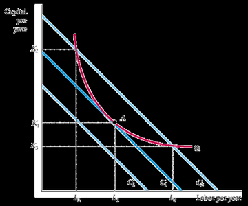
Isocost Lines

An isocost line shows all combinations of labor (L) and capital (K) that can be purchased for a given total cost, given input prices and :

• Equation:

• Slope: (shows the rate at which labor can be substituted for capital without changing total cost)

Example: If , , and , then describes the isocost line.

Cost-Minimizing Input Bundle

To minimize cost for a given output:

• Find the point where the isoquant (output level) is tangent to the isocost line (i.e., where )

• Ensure (the chosen bundle produces the desired output)

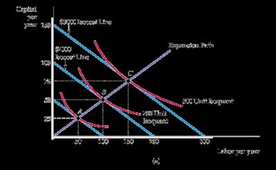
Graphical Solution and Examples

When both labor and capital are variable, the cost-minimizing bundle can be found graphically by identifying the tangency point between the isoquant for the desired output and the lowest possible isocost line.

Example: For , , to produce units, the optimal bundle is , .

• Similarly, ,

Expansion Path

The expansion path traces the cost-minimizing combinations of inputs as output increases, holding input prices constant. It connects the tangency points between isoquants and isocost lines for different output levels.

Long Run vs. Short Run Costs

• In the long run, there are no fixed costs:

• Long run costs are weakly lower than short run costs because firms have more flexibility in choosing input combinations.

Additional info: The flexibility in the long run allows firms to adjust all inputs, leading to more efficient production and lower average costs compared to the short run, where some inputs are fixed.