Production Technology and Producer Theory

Firms and Their Production Decisions

In microeconomics, firms use various factors of production—such as labor, capital, and materials—to produce goods and services. The production function describes the maximum output a firm can produce for any given combination of inputs, typically denoted as , where L is labor and K is capital.

• Short run: At least one input is fixed (e.g., capital).

• Long run: All inputs are variable; firms can adjust all factors of production.

• Fixed input: An input that cannot be changed in the short run (e.g., a factory building).

Example: In the short run, a firm may only be able to adjust labor, while capital remains fixed.

Production with One Variable Input (Labor)

When only labor is variable and capital is fixed, the production function simplifies to .

• Average Product of Labor (APL): Output per unit of labor input. Formula:

• Marginal Product of Labor (MPL): Additional output from one more unit of labor. Formula:

Example: If and is fixed at 1, then , , .

Visualizing APL and MPL

APL is the slope of the line connecting the origin to a point on the total product curve, while MPL is the slope of the tangent at that point.

Law of Diminishing Marginal Returns

As more units of a variable input (labor) are added to fixed inputs (capital), the additional output from each new unit eventually decreases. This is reflected in the flattening of the total product curve.

• Reason: Fixed capital limits the productivity of additional workers.

Identifying Diminishing Marginal Returns

To determine if a production curve exhibits diminishing marginal returns, observe whether the slope of the total product curve decreases as labor increases.

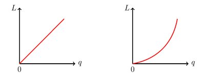
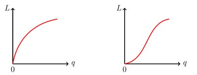
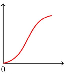
Example: Among several total product curves, the one where the slope decreases as labor increases demonstrates diminishing marginal returns.

Production with Two Variable Inputs

Isoquants and Isoquant Maps

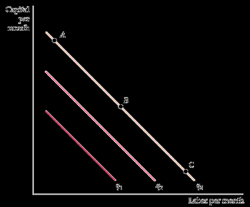
An isoquant is a curve representing all combinations of labor (L) and capital (K) that yield the same level of output. An isoquant map displays multiple isoquants, illustrating the flexibility of input combinations in production.

• Isoquant equation: For output level , all such that .

Example: An isoquant map shows how different combinations of labor and capital can produce output levels , , .

Marginal Rate of Technical Substitution (MRTS)

The MRTS measures the rate at which one input can be substituted for another while keeping output constant. It is the absolute value of the slope of an isoquant.

• Formula:

Example: If and , then (labor can replace capital at a 2:1 rate).

Types of Isoquant Maps

Isoquants can take different shapes depending on the substitutability of inputs:

• Smooth isoquants: Diminishing MRTS; inputs are imperfect substitutes.

• Perfect substitutes: Isoquants are straight lines; inputs can be substituted at a constant rate.

• Perfect complements: Isoquants are L-shaped; inputs must be used in fixed proportions.

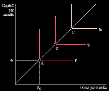
Example: In car manufacturing, tires and wheels are perfect complements; in some tasks, labor and machines may be perfect substitutes.

Returns to Scale

Definition and Types

Returns to scale describe how output changes as all inputs are increased proportionally:

• Increasing returns to scale: Output more than doubles when inputs are doubled.

• Constant returns to scale: Output exactly doubles when inputs are doubled.

• Decreasing returns to scale: Output less than doubles when inputs are doubled.

Example: Assembly lines often exhibit increasing returns to scale due to specialization; small businesses may face decreasing returns to scale due to management challenges.

Examples of Returns to Scale

• Constant returns to scale:

• Increasing returns to scale:

Additional info: Returns to scale are important for understanding firm growth and industry structure.