Demand and Supply: Foundations of Market Analysis

Law of Demand and Law of Supply

The Law of Demand states that, holding all else constant, when the price of a good increases, the quantity demanded decreases, and vice versa. This inverse relationship is fundamental to understanding consumer behavior. Conversely, the Law of Supply asserts that as the price of a good increases, the quantity supplied increases, indicating a direct relationship between price and quantity supplied.

• Law of Demand: ;

• Law of Supply: ;

• Demand Curve: Represents consumers' willingness to pay at each price point.

• Supply Curve: Represents the quantity firms are willing to supply at each price.

Changes in Demand and Supply

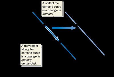
Change in Quantity Demanded vs. Change in Demand

A change in quantity demanded is caused solely by a change in the price of the good, resulting in movement along the demand curve. In contrast, a change in demand is caused by factors other than price, shifting the entire demand curve left or right.

• Change in Quantity Demanded: Movement along the curve due to price change.

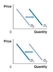
• Change in Demand: Shift of the entire curve due to non-price factors (e.g., income, tastes).

Factors Shifting Demand

Several factors can shift the demand curve:

• Income: Increase in income raises demand for normal goods and lowers demand for inferior goods.

• Prices of Related Goods: Substitutes and complements affect demand inversely or directly.

• Tastes and Preferences: Changes in consumer preferences can increase or decrease demand.

• Population Size: Larger populations increase demand.

Factors Shifting Supply

Supply can shift due to changes in:

• Input Prices: Higher input costs decrease supply.

• Technology: Technological improvements increase supply.

• Number of Firms: More firms increase market supply.

• Natural Events: Disasters can reduce supply.

Market Equilibrium

Equilibrium Price and Quantity

Market equilibrium occurs where the quantity demanded equals the quantity supplied. At this point, the market clears, and there is no tendency for price to change.

• Equilibrium Price (): The price at which .

• Equilibrium Quantity (): The quantity bought and sold at .

Surpluses and Shortages

If the market price is above equilibrium, a surplus occurs (quantity supplied exceeds quantity demanded). If the price is below equilibrium, a shortage occurs (quantity demanded exceeds quantity supplied). Market forces push the price toward equilibrium in both cases.

Shifts in Equilibrium

Changes in demand or supply shift the equilibrium price and quantity:

• Increase in Demand: Raises both equilibrium price and quantity.

• Increase in Supply: Lowers equilibrium price but increases equilibrium quantity.

Economic Efficiency and Surplus

Consumer and Producer Surplus

Consumer surplus is the difference between what consumers are willing to pay and what they actually pay. Producer surplus is the difference between the price producers receive and the minimum they are willing to accept.

• Consumer Surplus (CS):

• Producer Surplus (PS):

Deadweight Loss

Deadweight loss (DWL) is the reduction in total economic surplus that results from a market not being in competitive equilibrium, often due to price controls or taxes.

• At equilibrium: DWL = 0; total surplus is maximized.

• With price controls/taxes: DWL > 0; some surplus is lost.

Government Intervention: Price Floors, Price Ceilings, and Taxes

Price Floors and Price Ceilings

Governments may set price floors (minimum legal prices) or price ceilings (maximum legal prices) to influence market outcomes. These controls are only effective if set above (floor) or below (ceiling) the equilibrium price.

• Price Floor: Leads to surpluses if above equilibrium (e.g., minimum wage, agricultural supports).

• Price Ceiling: Leads to shortages if below equilibrium (e.g., rent control).

Taxes and Tax Incidence

When a tax is imposed, the burden is shared between buyers and sellers depending on the relative elasticities of demand and supply. The government collects tax revenue, but a deadweight loss is created due to reduced market activity.

• Tax Revenue: Area of the rectangle between the supply and demand curves at the new quantity.

• Deadweight Loss: Area of the triangle representing lost surplus from trades that no longer occur.

• Tax Incidence: The division of the tax burden between buyers and sellers.

Summary Table: Effects of Government Intervention

Key Formulas

• Consumer Surplus:

• Producer Surplus:

• Deadweight Loss: