Introduction to Microeconomics

Microeconomics is the study of individual decision-makers—consumers and producers—and their interactions in various market structures. The ECS2601 course covers foundational concepts, consumer and producer behavior, market dynamics, and the consequences of government intervention.

Elasticity

Types of Elasticity

Elasticity measures the responsiveness of one variable to changes in another, such as how quantity demanded or supplied responds to price changes.

• Price Elasticity of Demand (Ep): Measures the percentage change in quantity demanded for a 1% change in price.

• Income Elasticity: Measures how demand changes with income. Positive for normal goods, negative for inferior goods.

• Cross-Price Elasticity: Measures how demand for one good changes with the price of another. Positive for substitutes, negative for complements.

• Price Elasticity of Supply: Measures responsiveness of quantity supplied to price changes.

Point Elasticity is calculated at a specific point on the curve, while arc elasticity uses averages over a range.

Government Intervention: Price Controls

Governments may set ceiling prices (maximum prices) below equilibrium to make goods affordable, or floor prices (minimum prices) above equilibrium to support producers. These interventions can cause excess demand or supply, leading to market inefficiencies.

Consumer Behaviour

Consumer Preferences and Utility

Consumers are assumed to be rational, seeking to maximize satisfaction (utility) given their preferences and budget constraints. Preferences are modeled using indifference curves, which represent combinations of goods yielding equal satisfaction. Key assumptions include completeness, transitivity, and "more is better." The marginal rate of substitution (MRS) is the slope of the indifference curve, showing the rate at which a consumer is willing to trade one good for another.

Budget Constraints

The budget line represents all combinations of goods a consumer can afford given income and prices. Changes in income shift the budget line parallel, while changes in relative prices alter its slope.

Consumer Choice

Consumers maximize utility where the highest indifference curve is tangent to the budget line. The equilibrium condition is:

• (Marginal rate of substitution equals the price ratio)

Corner solutions occur when all income is spent on one good.

Marginal Utility and Consumer Choice

Marginal utility (MU) is the additional satisfaction from consuming one more unit. The equal marginal principle states that utility is maximized when the marginal utility per unit of expenditure is equal across goods:

Production Theory

Production Functions

Production describes how firms transform inputs (labour, capital) into outputs. The production function is , where is output, is capital, and is labour.

• Short Run: At least one input (usually capital) is fixed.

• Long Run: All inputs are variable.

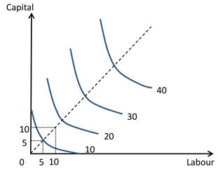
Isoquants

Isoquants are curves showing combinations of inputs that yield the same output, analogous to indifference curves in consumer theory. The marginal rate of technical substitution (MRTS) is the slope of the isoquant, indicating how much one input can be substituted for another while keeping output constant.

Returns to Scale

Returns to scale describe how output changes as all inputs are increased proportionally:

• Increasing Returns to Scale: Output increases more than inputs.

• Constant Returns to Scale: Output increases proportionally.

• Decreasing Returns to Scale: Output increases less than inputs.

The Cost of Production

Types of Costs

• Economic Cost: Includes explicit and implicit (opportunity) costs.

• Accounting Cost: Only explicit costs.

• Sunk Cost: Irrecoverable past expenditure.

• Total Cost (TC):

• Average Total Cost (ATC):

• Marginal Cost (MC):

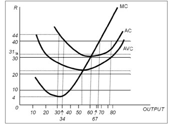
Short-Run Cost Curves

In the short run, marginal cost rises as output increases due to diminishing returns. The relationship between MC, ATC, and AVC is crucial for understanding firm behavior.

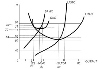
Long-Run Cost Curves

In the long run, firms can adjust all inputs. The long-run average cost (LRAC) and long-run marginal cost (LRMC) curves are envelopes of the short-run curves, reflecting optimal input combinations for each output level.

Profit Maximisation and Competitive Supply

Perfect Competition

In perfectly competitive markets, firms are price takers. The equilibrium condition for profit maximisation is:

• (Marginal revenue equals marginal cost)

• For competitive firms,

Firms continue producing as long as price covers average variable cost; otherwise, they shut down.

Short-Run and Long-Run Supply

• Short-Run Supply Curve: Portion of MC curve above AVC.

• Long-Run Supply Curve: Reflects entry and exit of firms, adjusting to zero economic profit.

Analysis of Competitive Markets

Consumer and Producer Surplus

Consumer surplus is the difference between what consumers are willing to pay and what they actually pay. Producer surplus is the difference between revenue and variable cost. These concepts are used to evaluate the effects of government policies, such as price controls, subsidies, and taxes.

Market Efficiency and Government Intervention

Competitive markets are efficient when they maximize aggregate surplus. Market failures can occur due to externalities or imperfect information, justifying government intervention.

Market Power: Monopoly and Monopsony

Monopoly

A monopolist is the sole supplier and faces the market demand curve. The equilibrium condition remains , but monopolists can set prices above marginal cost, leading to higher prices and lower quantities than in competitive markets. Monopoly power is measured by the Lerner Index:

Monopolies can cause deadweight loss and inefficiency, but natural monopolies may be regulated for public benefit.

Pricing with Market Power

Price Discrimination

Firms with market power may use price discrimination to capture consumer surplus:

• First-degree: Each consumer pays their reservation price.

• Second-degree: Prices vary by quantity purchased (block pricing).

• Third-degree: Different prices for different consumer groups.

Monopolistic Competition and Oligopoly

Monopolistic Competition

Many firms sell differentiated products with free entry. Firms earn economic profit in the short run, but entry drives profit to zero in the long run.

Oligopoly

Few firms dominate the market, often with strategic interactions. Models include Cournot (quantity competition), Stackelberg (leader-follower), Bertrand (price competition), and the Prisoner's Dilemma (collusion vs. competition).

Summary

This study guide provides a structured overview of microeconomic principles, including elasticity, consumer and producer behavior, production and cost theory, market structures, and the effects of government intervention. Understanding these concepts is essential for analyzing real-world economic issues and preparing for examinations in microeconomics.