Core Concepts in Microeconomics

Scarcity and Opportunity Cost

Scarcity is the fundamental economic problem of having limited resources to meet unlimited wants. Because resources are scarce, every choice involves an opportunity cost, which is the value of the next best alternative foregone when a decision is made.

• Scarcity: Limited resources versus unlimited wants.

• Opportunity Cost: The cost of the next best alternative given up.

• Example: Choosing to attend college means giving up potential income from working full-time.

Economic Models, Causation, and Correlation

Economists use economic models—simplified representations of reality—to analyze and predict economic behavior. It is important to distinguish between causation (one event causes another) and correlation (two events occur together but may not be causally related).

• Economic Model: A simplified framework for describing economic processes.

• Causation vs. Correlation: Causation implies a direct effect; correlation does not.

Optimization and Marginal Analysis

Economic agents make decisions by optimizing at the margin, weighing additional benefits against additional costs. The principle of diminishing marginal benefit states that as more of a good is consumed, the additional benefit from consuming an extra unit decreases.

• Optimization: Choosing the best feasible option given constraints.

• Marginal Analysis: Comparing marginal benefits and marginal costs.

• Diminishing Marginal Benefit: Each additional unit yields less benefit.

Demand, Supply, and Equilibrium

Demand

Demand refers to the quantity of a good or service that consumers are willing and able to purchase at various prices. The determinants of demand include income, prices of related goods, tastes, expectations, and the number of buyers.

• Law of Demand: As price falls, quantity demanded rises (ceteris paribus).

• Determinants: Income, prices of substitutes/complements, preferences, expectations, number of buyers.

Supply

Supply is the quantity of a good or service that producers are willing and able to sell at various prices. The determinants of supply include input prices, technology, expectations, and the number of sellers.

• Law of Supply: As price rises, quantity supplied rises (ceteris paribus).

• Determinants: Input prices, technology, expectations, number of sellers.

Market Equilibrium

Market equilibrium occurs where quantity demanded equals quantity supplied (QD = QS). At this point, the market clears, and there is no tendency for price to change.

• Solving for Equilibrium: Set QD = QS and solve for price and quantity.

• Example: If Qs = -14 + 40P and Qd = 286 - 20P, set Qs = Qd to find equilibrium.

Comparative Statics

Comparative statics analyzes the effects of changes in demand or supply on equilibrium in one market and potentially related markets.

• Example: An increase in demand for corn may affect the market for housing in a region due to resource reallocation.

Consumer Theory and Demand

Budget Line and Indifference Curves

The budget line shows all combinations of goods a consumer can afford. Its slope reflects the relative price of the two goods. Indifference curves represent combinations of goods that provide the consumer with the same level of satisfaction. The slope of the indifference curve is the marginal rate of substitution (MRS).

• Budget Line Equation:

• Indifference Curve: Downward sloping, convex to the origin.

Optimal Purchase Rule

The consumer's optimal choice occurs where the budget line is tangent to the highest attainable indifference curve. This is where the marginal utility per dollar is equalized across goods.

• Optimal Purchase Rule:

Deriving the Demand Curve

By varying the price of a good and observing the optimal quantity chosen, the individual demand curve can be derived. The optimal purchase rule explains why the demand curve slopes downward.

Elasticity

Price Elasticity of Demand

Elasticity of demand measures the responsiveness of quantity demanded to a change in price. The point elasticity formula is:

Arc elasticity (midpoint method) is:

Elasticity affects total revenue and profit. Other types include income elasticity of demand and cross-price elasticity of demand.

Elasticity Table

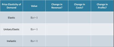
The following table summarizes the relationship between price elasticity of demand, revenue, costs, and profits:

Efficiency and Exchange

Consumer and Producer Surplus

Consumer surplus is the area above the price and below the demand curve, representing the net benefit to buyers. Producer surplus is the area above the supply curve (marginal cost) and below the price, representing the net benefit to sellers.

• Total Surplus: Consumer Surplus + Producer Surplus (+ tax revenue if applicable).

• Deadweight Loss: The loss in total surplus due to market interventions (e.g., taxes, price controls).

Example: For demand and supply , solve for equilibrium price and quantity, then calculate consumer and producer surplus. If a $2$ per unit tax is imposed, recalculate and determine deadweight loss.

Supply and Cost Structures

Production and Cost Concepts

• Total Physical Product (TPP): Total output produced by inputs.

• Marginal Physical Product (MPP):

• Diminishing Marginal Product: As more of an input is used, its marginal product eventually decreases.

• Marginal Revenue Product (MRP):

• Optimal Input Selection:

Cost Curves

• Total Cost (TC):

• Marginal Cost (MC):

• Average Cost (AC):

• Variable Cost (VC): Costs that vary with output.

• Average Variable Cost (AVC):

• Fixed Cost (FC): Costs that do not vary with output.

Revenue and Profit Maximization

• Total Revenue (TR):

• Marginal Revenue (MR):

• Profit Maximization: Choose Q such that

• Profit:

• Zero Profit Condition:

The Firm and the Industry: Perfect Competition

Characteristics of Perfect Competition

• Many buyers and sellers

• Homogeneous products

• Free entry and exit

• Perfect information

Short-Run and Long-Run Outcomes

• Short-run: Firms may earn positive, negative, or zero economic profits. No entry or exit occurs.

• Long-run: Entry and exit drive profits to zero. .

Industry and Firm Equilibrium

• Industry demand is downward sloping; firm faces a horizontal demand at market price.

• In the long run, supply shifts restore price to the minimum average cost.

Forms of Industrial Organization

Perfect Competition

• Advantages: Allocative and productive efficiency, consumer benefit from low prices.

• Disadvantages: Lack of product variety, limited innovation incentives.

Summary: Perfect competition leads to efficient outcomes in the long run, with zero economic profits and price equal to minimum average cost.