Master Formula Sheet

Key Microeconomics Formulas

This section summarizes the essential formulas used throughout microeconomics, providing definitions, context, and applications for each.

• Real Price Adjustment: Converts nominal prices to real prices using the Consumer Price Index (CPI) to account for inflation.

• Percent Change: Used for calculating elasticity and growth rates.

• Market Equilibrium: Equilibrium occurs where quantity demanded equals quantity supplied.

• Point Price Elasticity of Demand: Measures responsiveness at a specific point on the demand curve.

• Arc Elasticity: Used for large changes between two points.

• Income and Cross-Price Elasticity: Classifies goods as normal/inferior and substitutes/complements.

• Budget Line: Shows all affordable bundles for a consumer.

• Consumer Optimum: At the interior optimum, the marginal rate of substitution equals the price ratio.

• Market Demand: The sum of individual demands at each price.

• Consumer Surplus: Area under the demand curve and above the price paid.

• Slutsky Equation: Decomposes the total price effect into substitution and income effects.

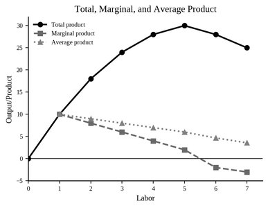
• Marginal and Average Product: Marginal product is extra output from one more unit; average product is output per worker.

• Marginal Rate of Technical Substitution (MRTS): Technical tradeoff between labor and capital.

• Returns to Scale: Classifies output response to scaling all inputs.

• Cobb-Douglas Returns: For Cobb-Douglas, add exponents to classify returns to scale.

• Cost-Minimization Connection: Choose input mix where MRTS equals input price ratio.

Chapter 2 - Supply and Demand

Market Model and Equilibrium

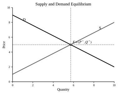
Supply and demand are the foundation of market analysis. The equilibrium price and quantity are determined where the supply and demand curves intersect.

• Demand Curve: Shows the relationship between price and quantity demanded, typically downward sloping.

• Supply Curve: Shows the relationship between price and quantity supplied, typically upward sloping.

• Equilibrium: The intersection of supply and demand curves determines the market price and quantity.

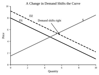
• Curve Shifts: Changes in demand or supply shift the respective curve, altering equilibrium.

Price Controls

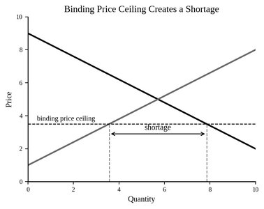
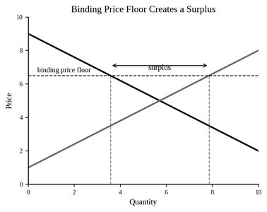
Government interventions such as price ceilings and floors affect market outcomes.

• Price Ceiling: A legal maximum price, binding if below equilibrium, creates a shortage.

• Price Floor: A legal minimum price, binding if above equilibrium, creates a surplus.

Elasticity

Elasticity measures how responsive quantity demanded or supplied is to changes in price, income, or other factors.

• Point Elasticity:

• Arc Elasticity:

• Total Revenue and Elasticity:

Chapter 3 - Consumer Behavior

Utility Maximization and Budget Constraints

Consumers choose the best affordable bundle by maximizing utility subject to their budget constraint.

• Utility Maximization: Occurs where the highest indifference curve is tangent to the budget line.

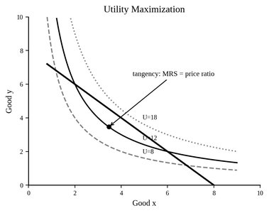
• Budget Line: Shows all affordable combinations of goods.

• Consumer Optimum:

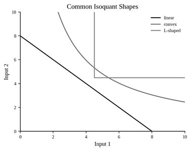
Indifference Curves

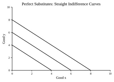
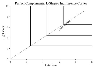
Indifference curves represent combinations of goods that yield the same utility.

• Perfect Substitutes: Straight-line indifference curves.

• Perfect Complements: L-shaped indifference curves.

Chapter 4 - Individual and Market Demand

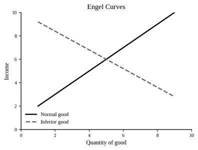
Price-Consumption and Engel Curves

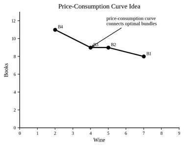
These curves illustrate how consumer choices change with price and income.

• Price-Consumption Curve: Connects optimal bundles as price changes.

• Engel Curve: Shows relationship between income and quantity demanded.

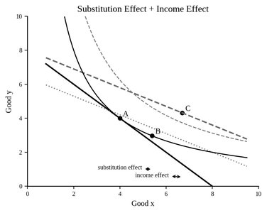
Income and Substitution Effects

When price changes, the total effect is split into substitution and income effects.

• Slutsky Equation:

• Graphical Decomposition:

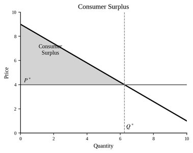
Consumer Surplus

Consumer surplus is the extra benefit consumers receive from paying less than their maximum willingness to pay.

• Consumer Surplus Formula:

• Triangle Area Shortcut:

• Consumer Surplus Graph:

Chapter 6 - Production

Production Function and Input Relationships

Firms use inputs to produce output, and the production function shows the maximum output possible from given inputs.

• Marginal and Average Product:

• Graph of Total, Marginal, and Average Product:

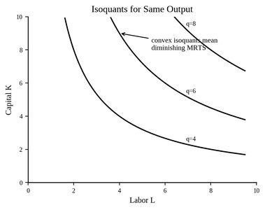
Isoquants and MRTS

Isoquants show combinations of inputs that yield the same output. MRTS measures the rate at which one input can be substituted for another.

• Isoquants:

• MRTS Formula:

• Isoquant Shapes:

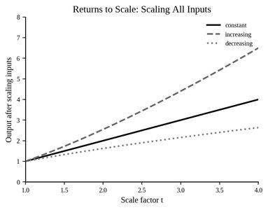
Returns to Scale

Returns to scale describe how output changes when all inputs are increased proportionally.

• Returns to Scale Formula:

• Returns to Scale Graph:

• Cobb-Douglas Production Function:

• Marginal Products in Cobb-Douglas:

Graph Interpretation Cheat Sheet

How to Read Microeconomic Graphs

• Step 1: Identify axes (e.g., price, quantity, income, input).

• Step 2: Identify what changed (e.g., price, income, technology).

• Step 3: Decide if the change is a movement along a curve or a shift/rotation.

• Step 4: Compare old and new points; state what happened to price, quantity, utility, output, or input use.

Common Graph Types: Supply and demand, budget line, indifference curve, Engel curve, demand curve, isoquant, total product curve, MP/AP curves.

Common Exam Traps: Confusing movement along a curve with a shift, misunderstanding diminishing returns, misinterpreting price controls, and misclassifying goods by elasticity signs.