Technology and Production

Definition of Technology

In microeconomics, technology refers to the processes a firm uses to turn inputs into outputs of goods and services. A technological change is any positive or negative change in a firm's ability to produce a given level of output with a given quantity of inputs.

• Inputs: Workers, machines, natural resources

• Outputs: Goods and services produced

• Positive technological change: Improved ability to turn inputs into outputs

The Short Run and the Long Run

Time Horizons in Production

Economists distinguish between the short run and the long run in production:

• Short run: At least one input is fixed (e.g., a factory lease).

• Long run: All inputs can be varied; firms can adopt new technology and change plant size.

The length of the long run varies by industry and firm.

Types of Costs

Fixed, Variable, and Total Costs

Costs are categorized based on their behavior with respect to output:

• Fixed costs (FC): Remain constant as output changes (e.g., rent, machinery).

• Variable costs (VC): Change as output changes (e.g., labor, raw materials).

• Total cost (TC): The sum of fixed and variable costs.

In the long run, all costs are variable.

Formula:

Explicit vs. Implicit Costs

Economists consider both explicit and implicit costs when analyzing firm decisions:

• Explicit cost: Involves direct monetary payment (e.g., wages, rent).

• Implicit cost: Nonmonetary opportunity cost (e.g., foregone salary, interest, depreciation).

Both types of costs are real and affect economic profit.

Production Functions and Cost Tables

Short-Run Production Function

The production function shows the relationship between inputs employed and the maximum output that can be produced. For example, Jill's restaurant uses pizza ovens (fixed input) and workers (variable input) to produce pizzas.

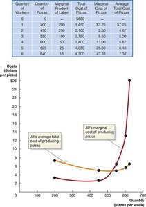
Cost Table Example

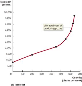
Graphing Total Cost

The total cost curve shows how total cost increases as output increases. Fixed costs ensure that total cost is not zero when output is zero.

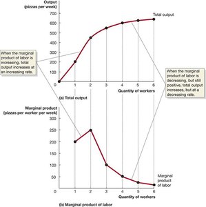
Marginal and Average Product of Labor

Definitions

• Marginal product of labor (MPL): The additional output produced by hiring one more worker.

• Average product of labor (APL): Total output divided by the number of workers.

Specialization can increase MPL initially, but eventually, diminishing returns set in.

Law of Diminishing Returns

The law of diminishing returns states that adding more of a variable input to the same amount of a fixed input will eventually cause the marginal product of the variable input to decline.

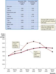
Average and Marginal Product Relationship

If the marginal product is above the average product, the average rises; if below, the average falls. This is analogous to how semester GPA affects cumulative GPA.

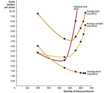
Short-Run Costs: Marginal and Average Costs

Definitions and Formulas

• Marginal cost (MC): The change in total cost from producing one more unit of output.

• Average total cost (ATC): Total cost divided by output.

• Average fixed cost (AFC): Fixed cost divided by output.

• Average variable cost (AVC): Variable cost divided by output.

Formulas:

Cost Curves and Their Shapes

Cost curves typically exhibit a U-shape due to the law of diminishing returns. Marginal cost intersects average total cost and average variable cost at their minimum points.

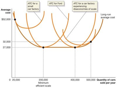
Long-Run Costs and Economies of Scale

Long-Run Average Cost Curve

In the long run, all inputs are variable, and the long-run average cost (LRAC) curve shows the lowest possible cost to produce each output level when all inputs can be adjusted.

Economies and Diseconomies of Scale

• Economies of scale: LRAC falls as output increases due to factors like specialization and bulk purchasing.

• Minimum efficient scale: The lowest output level at which economies of scale are exhausted.

• Constant returns to scale: LRAC remains unchanged as output increases.

• Diseconomies of scale: LRAC rises as output increases, often due to management inefficiencies.

Isoquants and Isocosts: Input Choice and Cost Minimization

Isoquants

An isoquant shows all combinations of two inputs (e.g., labor and capital) that produce the same level of output. Higher isoquants represent higher output levels.

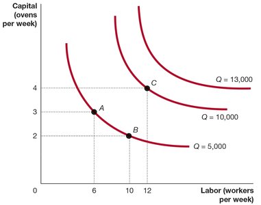
Marginal Rate of Technical Substitution (MRTS)

The MRTS is the rate at which a firm can substitute one input for another while keeping output constant. It is the slope of the isoquant and typically diminishes as more of one input is used.

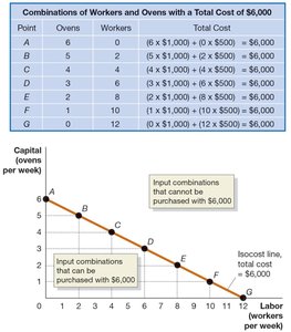
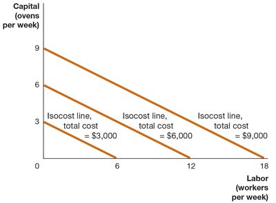
Isocost Lines

An isocost line shows all combinations of two inputs that have the same total cost. The slope of the isocost line is determined by the ratio of input prices.

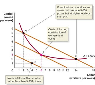
Cost Minimization

The cost-minimizing combination of inputs occurs where an isoquant is tangent to an isocost line. At this point, the MRTS equals the ratio of input prices:

where and are the marginal products of labor and capital, and and are their respective prices.

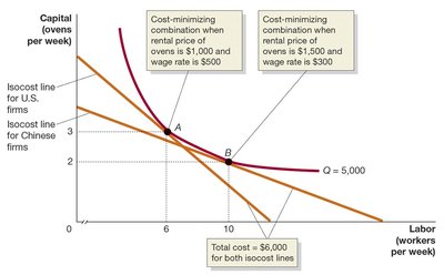
Effect of Input Price Changes

Changes in input prices shift the isocost line and alter the cost-minimizing input combination.

Application: Efficiency in the NFL

Economic efficiency requires that resources (e.g., player salaries) be allocated according to marginal product. Studies show that NFL teams sometimes overpay for early draft picks, indicating inefficiency.

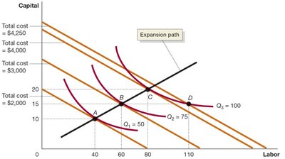
Expansion Path

The expansion path traces the cost-minimizing combinations of inputs as a firm expands output in the long run, holding input prices constant.

Summary Table: Key Cost Definitions