Sellers and Incentives in Perfect Competition: Production, Costs, and Profit Maximization

Study Guide - Smart Notes

Tailored notes based on your materials, expanded with key definitions, examples, and context.

Ch. 6 Sellers and Incentives

6.1 Sellers in a Perfectly Competitive Market

In a perfectly competitive market, sellers operate under specific conditions that shape their incentives and behavior. Understanding these conditions is crucial for analyzing firm decisions and market outcomes.

No buyer or seller is large enough to influence the market price. Each participant is a price taker.
Sellers produce identical goods. Products are homogeneous, so buyers are indifferent between sellers.
Free entry and exit. Firms can freely enter or leave the market, ensuring long-run equilibrium.

Example: The Wisconsin Cheeseman produces boxes of cheese in a competitive market.

Factory floor with production lines

6.2 The Seller’s Problem

Firms aim to maximize profit by solving three key problems:

How to make the product: Transforming inputs into outputs efficiently.
What is the cost of making the product? Calculating costs associated with production.
How much can the seller get for the product? Determining revenue based on market price.

Production: Inputs to Outputs

Short run: Some inputs are fixed and cannot be changed (e.g., factory size).
Long run: All inputs can be varied (e.g., expanding production facilities).
Variable factor of production: Inputs that can be changed in the short run (e.g., labor).
Fixed factor of production: Inputs that remain constant in the short run (e.g., machinery).

Marginal Product and Diminishing Returns

The marginal product is the additional output generated by adding one more unit of a variable input, such as labor. As more workers are hired, the marginal product typically increases at first, then decreases due to diminishing marginal product.

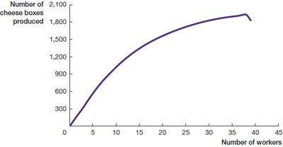
Short-run production function for cheese boxes

Example: Wisconsin Cheeseman's production data shows output per day and marginal product for each additional worker.

Number of Workers	Output per Day	Marginal Product
1	100	100
2	207	107
3	321	114
4	444	123
5	558	114
6	664	106
7	762	98
8	854	92
9	939	85
10	1019	80

Additional info: Diminishing marginal product is analogous to diminishing marginal utility in consumer theory.

6.3 From the Seller’s Problem to the Supply Curve

Understanding costs is essential for deriving the supply curve. Firms analyze various cost measures to determine optimal output.

Cost Concepts

Total Cost (TC): Sum of variable and fixed costs.
Variable Cost (VC): Costs that change with output.
Fixed Cost (FC): Costs that remain constant in the short run.
Marginal Cost (MC): Change in total cost from producing one more unit.
Average Variable Cost (AVC):
Average Total Cost (ATC):

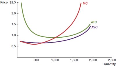
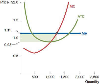
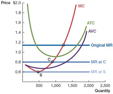
Marginal cost, average total cost, and average variable cost curves

Example: Cost curves for Wisconsin Cheeseman illustrate how MC, ATC, and AVC change with output.

6.4 Profit Maximization

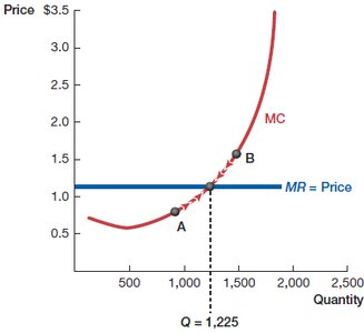
Firms maximize profit by choosing the output level where marginal revenue equals marginal cost (). In perfect competition, price equals marginal revenue ().

Total Revenue (TR):
Profit:
Profit maximization rule: Produce where

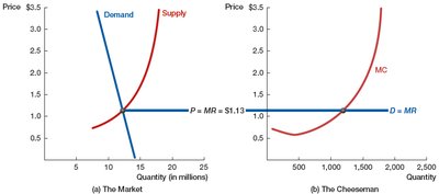
Supply and demand: market vs. individual firm

Example: The Cheeseman maximizes profit at the quantity where .

Profit maximization at MR = MC

Profit calculation:

Profit area between price and ATC

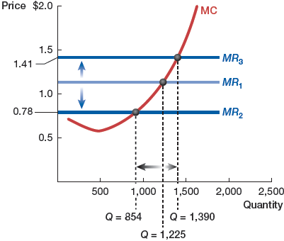
How output changes as price changes: Higher prices increase profit-maximizing output; lower prices decrease it.

Effect of price changes on profit-maximizing output

Additional info: Economic profit includes opportunity costs, while accounting profit considers only explicit costs.

6.5 From the Short Run to the Long Run

Firms' shutdown decisions differ between the short run and long run. In the short run, firms must cover variable costs; in the long run, they must cover total costs.

Short-run shutdown condition:
Long-run shutdown condition:

Shutdown points and profit conditions

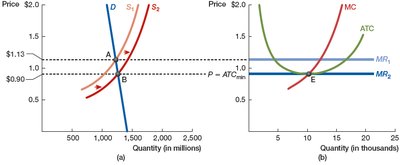
Long-run equilibrium: In the long run, free entry and exit ensure that firms earn zero economic profit, and price equals minimum average cost ().

Long-run price and entry/exit

All costs are variable in the long run. Firms can adjust all inputs and scale production.

Long-run adjustment and costs

Short- and long-run supply curves: The shape of the long-run ATC curve is determined by economies of scale.

Long-run ATC and supply curves

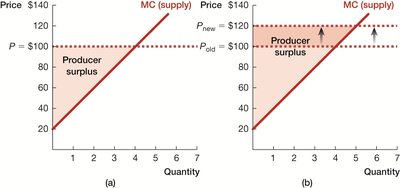
6.6 Producer Surplus

Producer surplus is the difference between the market price and the minimum price a firm would accept (represented by the supply curve or MC curve). It measures the benefit to producers from participating in the market.

Producer surplus: Area below market price and above supply (MC) curve.
Calculation: For a triangle,

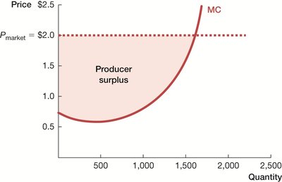
Producer surplus area below price and above MC Producer surplus for trucking services

Example: If the base is 4 and height is $80, producer surplus is $60.

Economies of Scale and Average Cost

Economies of scale describe how average total cost (ATC) changes as output increases:

Economies of scale: ATC falls as output increases (increasing returns to scale).
Constant returns to scale: ATC remains unchanged as output increases.
Diseconomies of scale: ATC rises as output increases (decreasing returns to scale).

Reasons: Large set-up costs, worker specialization, and management inefficiencies.

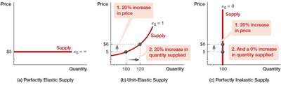
Elasticity of Supply

Elasticity of supply measures how responsive quantity supplied is to changes in price.

Elastic supply: ; quantity supplied is very responsive to price changes.
Inelastic supply: ; quantity supplied changes less than price.
Unit-elastic supply: ; percentage change in quantity equals percentage change in price.

Factors affecting elasticity: Inventory levels, ease of hiring workers, and time horizon.

Elasticity of supply: perfectly elastic, unit-elastic, and perfectly inelastic

Additional info: Elasticity of supply is not typically tested on midterm exams but is important for understanding market dynamics.