Chapter 11: Types of Goods and Market Failures

Classification of Goods

Goods can be categorized based on two criteria: excludability (whether people can be prevented from using the good) and rivalry in consumption (whether one person's use reduces another's ability to use it). This classification helps explain why markets sometimes fail to provide efficient outcomes.

• Private Goods: Excludable and rival (e.g., food, clothing).

• Public Goods: Non-excludable and non-rival (e.g., national defense).

• Common Resources: Non-excludable but rival (e.g., fish in the ocean).

• Club Goods: Excludable but non-rival (e.g., cable TV).

Example: Roads can be categorized differently depending on congestion and tolls (Active Learning: Categorizing roads).

Market Failures and Externalities

When goods are not excludable, markets may fail to provide the efficient quantity. Public goods create positive externalities (benefits to others), while common resources create negative externalities (costs to others).

• Public Goods: Suffer from the free-rider problem, where individuals benefit without paying, leading to under-provision.

• Common Resources: Suffer from the Tragedy of the Commons, where overuse leads to depletion.

Example: National defense is under-provided by the market because no one can be excluded from its benefits.

Government Solutions

When property rights are not well established, government intervention can improve outcomes:

• Issuing pollution permits to assign property rights.

• Selling hunting permits to prevent overuse of wildlife.

• Using tax revenue to provide public goods like national defense.

Case Study: The extinction of elephants in Africa was addressed by assigning property rights, incentivizing conservation.

Chapter 14: Costs of Production

Economic vs. Accounting Profit

Accounting profit is total revenue minus explicit costs. Economic profit also subtracts implicit costs (opportunity costs of resources).

• Formula:

Short Run vs. Long Run

The distinction is based on the flexibility of inputs:

• Short Run: At least one input is fixed (e.g., land).

• Long Run: All inputs are variable.

Production and Cost Relationships

As more workers are added to a fixed input, the marginal product of labor (MPL) diminishes, making the total cost curve steeper as output increases.

• Fixed Costs (FC): Do not vary with output.

• Variable Costs (VC): Vary with output.

• Total Cost (TC):

• Average Total Cost (ATC):

• Marginal Cost (MC): The increase in total cost from producing one more unit.

Cost Curves and Their Shapes

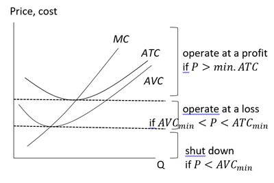
The ATC curve is U-shaped due to the interplay between Average Fixed Cost (AFC) and Average Variable Cost (AVC). The MC curve intersects the ATC and AVC curves at their minimum points.

• If MC < ATC, ATC is falling.

• If MC > ATC, ATC is rising.

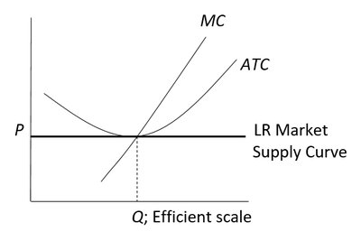
• The output that minimizes ATC is called the efficient scale of the firm.

Long-Run Average Total Cost (LRATC)

The LRATC curve is U-shaped due to:

• Economies of Scale: ATC falls as output increases (at low Q).

• Diseconomies of Scale: ATC rises as output increases (at high Q).

• Constant Returns to Scale: ATC is constant as output increases (at medium Q).

Example: Large factories may have lower costs per unit due to specialization, but very large firms may face management inefficiencies.

Chapter 15: Market Model – Perfect Competition

Firm Behavior in Perfect Competition

In a perfectly competitive market, firms are price takers. The price is determined by the market, and each firm can sell as much as it wants at that price.

• Average Revenue (AR):

• Marginal Revenue (MR): For a competitive firm,

• Profit Maximization: Produce Q where (which is for a competitive firm).

Short-Run Decisions

• A firm will shut down temporarily if .

• A firm will operate at a loss if .

• A firm will operate at a profit if .

Profit Calculation

• Profit ():

Long-Run Decisions and Market Supply

• Firms enter the market if and exit if .

• In the long run, firms earn zero economic profit: at the efficient scale.

• The long-run market supply curve is horizontal at (if all firms have identical costs and input prices are constant).

Market Adjustments

• In the short run, the number of firms is fixed due to fixed costs, so firms can earn positive or negative economic profit.

• In the long run, free entry and exit ensure zero economic profit and efficient allocation of resources.

• If demand increases, new firms enter, increasing market quantity but not price (in the constant-cost case).

• In reality, the long-run supply curve may slope upward if input costs rise or firms have different costs.

Summary Table: Short-Run and Long-Run Firm Decisions

Additional info: The images included reinforce the graphical relationships between cost curves and firm decisions in perfect competition, as well as the determination of the long-run market supply curve at the efficient scale.