 Back
BackTechnology, Production, and Costs: Microeconomics Study Guide
Study Guide - Smart Notes
 Tailored notes based on your materials, expanded with key definitions, examples, and context.
Technology, Production, and Costs
Introduction
This unit explores how firms use technology and inputs to produce goods and services, analyzes the relationship between production and costs, and examines the concepts of short-run and long-run costs. Understanding these principles is essential for analyzing firm behavior and market outcomes in microeconomics.
Technology: An Economic Definition
Technology in economics refers to the processes a firm uses to turn inputs into outputs. It encompasses not only machinery and equipment but also managerial skills, worker training, and organizational efficiency.
Technology: The set of processes used to convert inputs (labor, capital, natural resources) into outputs (goods and services).
Technological change: A positive or negative change in a firm's ability to produce a given level of output with a given quantity of inputs.
Example: A pizza restaurant's technology includes oven capacity, cook speed, and managerial organization.
Positive technological change: Producing more output with the same inputs or the same output with fewer inputs.
Negative technological change: Reduced output due to less-skilled workers or damaged facilities.
The Short Run and the Long Run in Economics
Firms distinguish between the short run and the long run when analyzing production and costs.
Short run: At least one input is fixed (e.g., capital).
Long run: All inputs are variable; firms can adopt new technology and change plant size.
Example: A pizza restaurant may add ovens in a few weeks, while an automobile factory may take years to expand.
The Difference Between Fixed Costs and Variable Costs
Costs are categorized as fixed or variable depending on whether they change with output.
Total cost (TC): The sum of all inputs used in production.
Variable costs (VC): Costs that change as output changes (e.g., labor, raw materials).
Fixed costs (FC): Costs that remain constant as output changes (e.g., rent, insurance).
Formula:
Implicit Costs Versus Explicit Costs
Opportunity cost is the value of the next best alternative forgone. Costs are either explicit (monetary) or implicit (nonmonetary).
Explicit cost: Involves spending money (e.g., wages, rent).
Implicit cost: Nonmonetary, such as forgone salary or interest.
Economic depreciation: The reduction in value of capital over time.
Example: Jill's forgone salary and interest, plus depreciation, are implicit costs.
The Production Function
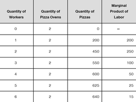
The production function shows the relationship between inputs and maximum output. In the short run, some inputs are fixed.
Production function: Relationship between inputs employed and maximum output produced.
Short-run production: Only variable inputs (e.g., labor) can be changed.
Quantity of Workers | Quantity of Pizza Ovens | Quantity of Pizzas | Marginal Product of Labor |
|---|---|---|---|
0 | 2 | 0 | – |
1 | 2 | 200 | 200 |
2 | 2 | 450 | 250 |
3 | 2 | 550 | 100 |
4 | 2 | 600 | 50 |
5 | 2 | 625 | 25 |
6 | 2 | 640 | 15 |
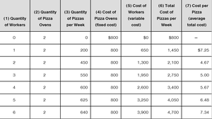
A First Look at the Relationship between Production and Cost
Costs can be calculated based on the number of workers and ovens required to produce a given quantity of pizzas.
Quantity of Workers | Quantity of Ovens | Quantity of Pizzas per Week | Cost of Pizza Ovens (fixed cost) | Cost of Workers (variable cost) | Total Cost of Pizzas per Week | Cost per Pizza (average total cost) |
|---|---|---|---|---|---|---|
0 | 2 | 0 | $800 | $0 | $800 | – |
1 | 2 | 200 | $800 | $650 | $1,450 | $7.25 |
2 | 2 | 450 | $800 | $1,300 | $2,100 | $4.67 |
3 | 2 | 550 | $800 | $1,950 | $2,750 | $5.00 |
4 | 2 | 600 | $800 | $2,600 | $3,400 | $5.67 |
5 | 2 | 625 | $800 | $3,250 | $4,050 | $6.48 |
6 | 2 | 640 | $800 | $3,900 | $4,700 | $7.34 |
The Marginal Product of Labor and the Average Product of Labor
The marginal product of labor is the additional output from hiring one more worker. The average product of labor is total output divided by the number of workers.
Marginal product of labor: Additional output from one more worker.
Average product of labor: Total output divided by number of workers.
Division of labor: Dividing tasks increases productivity.
Specialization: Workers focus on specific tasks, increasing efficiency.
The Law of Diminishing Returns
At some point, adding more of a variable input to a fixed input causes the marginal product to decline.
Law of diminishing returns: Adding more labor to fixed capital eventually decreases marginal product.
Example: Marginal product declines after hiring the third worker.
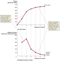
Graphing Production
Production and marginal product can be visualized graphically. Output increases at an increasing rate initially, then at a decreasing rate due to diminishing returns.
The Relationship Between Marginal Product and Average Product
The average product of labor is the average of marginal products. When marginal product exceeds average product, average product rises; when it is less, average product falls.
Average product of labor:
Marginal product equals average product: At the maximum average product.
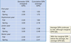
An Example of Marginal and Average Values: College Grades
The relationship between marginal and average values applies to other variables, such as GPA.
Semester GPA (marginal GPA) | Cumulative GPA (average GPA) |
|---|---|
1.50 | 1.50 |
2.00 | 1.75 |
2.20 | 1.90 |
3.00 | 2.18 |
3.20 | 2.38 |
3.00 | 2.48 |
2.40 | 2.47 |
2.00 | 2.41 |
The Relationship Between Short-Run Production and Short-Run Cost
Technology determines marginal and average products, which affect costs. Marginal cost is the change in total cost from producing one more unit.
Marginal cost (MC):
When marginal product rises, marginal cost falls; when marginal product falls, marginal cost rises.
Marginal cost curve is U-shaped.
Why are the Marginal and Average Cost Curves U Shaped?
Marginal cost falls when marginal product rises and rises when marginal product falls, creating a U-shaped curve. Average total cost also has a U shape.
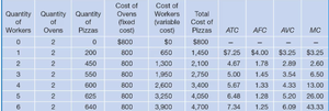
Graphing Cost Curves
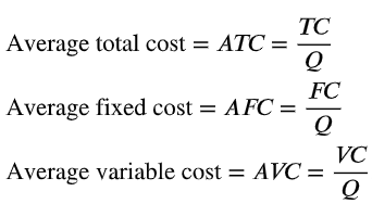
Cost curves are important for understanding firm behavior. Average fixed cost, average variable cost, and average total cost are calculated as follows:
Average total cost (ATC):
Average fixed cost (AFC):
Average variable cost (AVC):
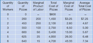
Quantity of Workers | Quantity of Pizzas | Marginal Product of Labor | Total Cost of Pizzas | Marginal Cost of Pizzas | Average Total Cost of Pizzas |
|---|---|---|---|---|---|
0 | 0 | – | $800 | – | – |
1 | 200 | 200 | $1,450 | $3.25 | $7.25 |
2 | 450 | 250 | $2,100 | $2.60 | $4.67 |
3 | 550 | 100 | $2,750 | $6.50 | $5.00 |
4 | 600 | 50 | $3,400 | $13.00 | $5.67 |
5 | 625 | 25 | $4,050 | $26.00 | $6.48 |
6 | 640 | 15 | $4,700 | $43.33 | $7.34 |
Costs in the Long Run
In the long run, all costs are variable. Firms can adjust all inputs and choose the most efficient scale of production.
Long-run average cost curve: Shows the lowest cost at which a firm can produce a given quantity of output when no inputs are fixed.
Economies of scale: Long-run average cost falls as output increases.
Diseconomies of scale: Long-run average cost rises as output increases beyond a certain point.
Minimum efficient scale: The lowest level of output at which a firm can minimize long-run average cost.
Summary Table: Cost Concepts
Cost Concept | Definition | Formula |
|---|---|---|
Total Cost (TC) | Sum of all costs | |
Average Total Cost (ATC) | Total cost per unit | |
Average Fixed Cost (AFC) | Fixed cost per unit | |
Average Variable Cost (AVC) | Variable cost per unit | |
Marginal Cost (MC) | Cost of one more unit |
Additional info: All tables and graphs are reconstructed from the provided images and text for clarity and completeness.
