2D Kinematics

Vector Displacement, Velocity, and Acceleration

In two-dimensional motion, displacement, velocity, and acceleration are all vector quantities, meaning they have both magnitude and direction. Understanding their components is essential for analyzing motion in a plane.

• Displacement (\( \Delta \vec{r} \)): The change in position of an object, with x- and y-components.

• Velocity (\( \vec{v} \)): The rate of change of displacement. The instantaneous velocity is tangent to the path, while the average velocity is parallel to the overall displacement.

• Acceleration (\( \vec{a} \)): The rate of change of velocity, also with x- and y-components.

Key equations:

• \( \Delta \vec{r} = \vec{r}_2 - \vec{r}_1 \)

• \( \vec{v} = \frac{\Delta \vec{r}}{\Delta t} \)

• \( \vec{a} = \frac{\Delta \vec{v}}{\Delta t} \)

Example: If a vector has components \( K_x = 6 \) m and \( K_y = -8 \) m, its magnitude is \( K = \sqrt{K_x^2 + K_y^2} = 10 \) m, and the angle with the +x axis is \( \theta = \tan^{-1}\left(\frac{K_y}{K_x}\right) = -53^\circ \).

Vectors in 2D Motion

Component Analysis and Direction

Vectors can be resolved into x and y components using trigonometric functions. The sign of each component depends on the vector's direction relative to the coordinate axes.

• Component Formulas:

  • \( A_x = A \cos \theta \)

  • \( A_y = A \sin \theta \)

• Signs of Components: Determined by the quadrant in which the vector lies.

Example: For a vector at an angle \( \theta \) relative to the -y axis, the length of the adjacent side is \( A \cos \theta \).

Projectile Motion

Basic Principles and Assumptions

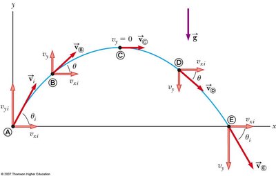
Projectile motion describes the motion of an object launched into the air, subject only to gravity (assuming air resistance is negligible). The path followed is a parabola, called the trajectory.

• The acceleration due to gravity (\( \vec{g} \)) is constant and directed downward (\( 9.80 \) m/s2).

• Horizontal and vertical motions are independent of each other.

• Kinematic equations can be applied separately to the x and y directions.

Kinematic Equations for Projectile Motion

The following equations describe the motion in each direction:

• Horizontal (x-direction):

  • \( v_{xf} = v_{xi} + a_x \Delta t \) (usually \( a_x = 0 \))

  • \( \Delta x = v_{xi} \Delta t + \frac{1}{2} a_x \Delta t^2 \)

  • \( v_{xf}^2 = v_{xi}^2 + 2 a_x \Delta x \)

  • \( \Delta x = \frac{1}{2} (v_{xf} + v_{xi}) \Delta t \)

• Vertical (y-direction):

  • \( v_{yf} = v_{yi} + a_y \Delta t \)

  • \( \Delta y = v_{yi} \Delta t + \frac{1}{2} a_y \Delta t^2 \)

  • \( v_{yf}^2 = v_{yi}^2 + 2 a_y \Delta y \)

  • \( \Delta y = \frac{1}{2} (v_{yf} + v_{yi}) \Delta t \)

Analyzing Projectile Motion

To solve projectile motion problems:

1. Resolve the initial velocity into x and y components:

   • \( v_{xi} = v_i \cos \theta \)

   • \( v_{yi} = v_i \sin \theta \)

2. Apply kinematic equations to each direction separately.

3. Use the time of flight (\( \Delta t \)) as the link between x and y motions.

Example: A rock is thrown from a castle wall with \( v_i = 12 \) m/s at \( 42^\circ \) above horizontal, landing 9.5 m below the starting height. The final velocity just before landing is found by:

• \( v_{xi} = 12 \cos 42^\circ = 8.9 \) m/s

• \( v_{yi} = 12 \sin 42^\circ = 8.0 \) m/s

• \( v_{yf}^2 = v_{yi}^2 + 2 a_y \Delta y \)

• \( v_{yf} = -15.8 \) m/s (downward)

• Total speed: \( v = \sqrt{v_{xi}^2 + v_{yf}^2} = 18.1 \) m/s

• Direction: \( \theta = \tan^{-1}\left(\frac{v_{yf}}{v_{xi}}\right) = -61^\circ \) (below horizontal)

Graphical Analysis of Projectile Motion

Position vs. time graphs for projectile motion are parabolic. The direction of velocity and acceleration at any point can be inferred from the slope and curvature of the graph.

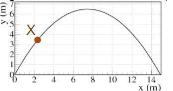
Example: At point X, the velocity vector is tangent to the curve, and the acceleration vector always points downward due to gravity.

Uniform Circular Motion

Concepts and Characteristics

In uniform circular motion, an object moves at constant speed along a circular path. Although the speed is constant, the direction of the velocity changes continuously, resulting in a nonzero acceleration called centripetal acceleration.

• Centripetal acceleration always points toward the center of the circle.

• Magnitude: \( a_c = \frac{v^2}{r} \), where \( v \) is speed and \( r \) is the radius of the circle.

Example: A merry-go-round horse travels at constant speed around a circle of circumference 31.4 m in 20.0 s. The velocity at any point is tangent to the circle, and the average acceleration from one point to another can be found using the change in velocity vectors over the time interval.

Summary Table: Key Quantities in 2D Motion

Common Projectile Motion Questions

• What is the final height (\( y_{final} \))?

• What is the initial velocity (\( v_{initial} \))?

• What angle (\( \theta \)) is needed for a given range?

• What is the peak height (\( y_{max} \))?

• What is the time of flight (\( \Delta t \))?

• What is the maximum distance (\( \Delta x \))?

• What is the final speed (magnitude and direction)?

Solving these questions involves breaking the motion into x and y components, applying the appropriate kinematic equations, and using the relationships between the variables.

Additional info: The notes above expand on the brief lecture points, providing definitions, equations, and examples for clarity and completeness. The included images directly illustrate projectile motion and its graphical analysis, reinforcing the concepts discussed.