Kinematics: How to Think About Motion

Physical Models and Their Purpose

Physical models are simplified representations of real systems, designed to make complex phenomena more manageable and understandable. In physics, we often start with simple models and add complexity only as needed. This approach allows us to focus on essential features and develop intuition before tackling more intricate scenarios.

• Physical Model: A simplified version of a real system, often ignoring size, shape, or other details.

• Mathematical Model: Uses equations and mathematical relationships to predict or explain physical behavior.

• Application: Modelling objects as points and analyzing their motion along a straight line.

Structure of Kinematics

Kinematics is the study of motion without considering its causes. It focuses on describing how objects move using physical quantities such as position, velocity, and acceleration. Multiple representations—stories, diagrams, graphs, and equations—can describe the same motion, and understanding their relationships is key to problem solving.

• Physical Quantities: Position, velocity, acceleration, displacement, and time.

• Relationships: Rates of change, slopes, and derivatives connect these quantities.

• Representations: Words, diagrams, graphs, and equations.

• Expert Approach: Choose origin and positive direction, sketch graphs, and use appropriate mathematical descriptions.

Signs and Coordinate Systems

Choosing a coordinate system and sign convention is fundamental in kinematics. The origin and positive direction must be defined and consistently used throughout the problem.

• Origin: Reference point for position measurements.

• Positive Direction: Direction chosen as positive for displacement and velocity.

• Consistency: Maintain the same convention throughout the analysis.

Motion Diagrams and Kinematic Graphs

Motion diagrams visually represent the position of an object at regular time intervals. These diagrams can be translated into kinematic graphs, where the slope of the position-time graph gives velocity, and the slope of the velocity-time graph gives acceleration.

• Position-Time Graph: Slope represents velocity.

• Velocity-Time Graph: Slope represents acceleration.

• Acceleration-Time Graph: Area under the curve represents change in velocity.

Key Kinematic Equations

Calculus provides precision in kinematics, allowing us to relate position, velocity, and acceleration through derivatives and integrals.

• Velocity as derivative of position:

• Acceleration as derivative of velocity:

• Velocity as integral of acceleration:

• Position as integral of velocity:

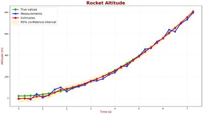
Example: Calculus in Kinematics

Consider a rocket whose altitude is given by . The instantaneous vertical velocity is found by differentiating the altitude with respect to time:

• Instantaneous velocity:

Piecewise Motion and Problem Solving

Piecewise Motion Example

When an object's motion changes over time, it is often described using piecewise functions. Each segment has its own velocity and acceleration expressions, and values at the boundaries must be consistent.

• Velocity function:

• Position function: (initial position)

• Boundary values: Ensure position and velocity are continuous at transition points.

Free Fall Example

Consider a shotputter accelerating a shot upward from rest. The motion is described by different equations before and after release, using integration to find velocity and height.

• Acceleration:

• Velocity:

• Position:

Final Advice for Kinematics Problem Solving

• Draw diagrams before solving.

• Establish a coordinate system and sign convention.

• Ensure positions and velocities are consistent at motion changes.

• Use multiple representations (diagrams, graphs, equations) to fully understand the problem.