One-Dimensional Kinematics

Introduction to Kinematics

Kinematics is the branch of mechanics that describes the motion of objects without considering the causes of motion. In one-dimensional kinematics, we analyze motion along a straight line, typically using a coordinate system with a defined origin and positive direction.

• Coordinate System: Essential for describing motion; defines the origin and direction (e.g., +x direction).

• SI Units: The standard unit for distance and displacement is the meter (m).

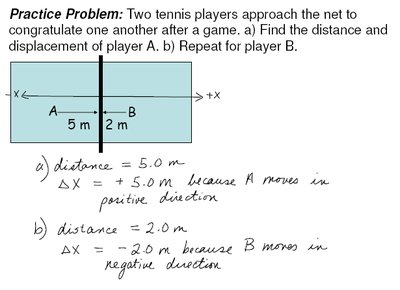
Distance and Displacement

Distance and displacement are fundamental concepts in describing motion:

• Distance: The total length traveled by an object, regardless of direction. Always positive.

• Displacement (\( \Delta x \)): The change in position, calculated as final position minus initial position. Displacement can be positive or negative, depending on direction.

Formula:

Example: If you drive from your house to the grocery store and back, your distance is the total path traveled, while your displacement is zero (since you return to your starting point).

Average Speed and Average Velocity

Speed and velocity are measures of how fast an object moves, but velocity includes direction:

• Average Speed (\( v_{\text{av}} \)): Total distance divided by elapsed time. Always positive.

• Average Velocity (\( v_{\text{av}} \)): Displacement divided by elapsed time. Can be positive or negative.

Formulas:

Example: If you return to your starting point, your average velocity is zero, but your average speed is not.

Graphical Interpretation of Motion

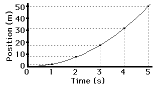
Graphs are powerful tools for visualizing motion. The slope of a position vs. time graph gives velocity, while the slope of a velocity vs. time graph gives acceleration.

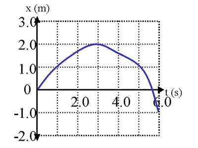
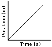
• Position vs. Time: Slope represents velocity.

• Velocity vs. Time: Slope represents acceleration; area under the curve gives displacement.

Instantaneous Velocity

Instantaneous velocity is the velocity at a specific instant. It is found as the slope of the tangent to the position vs. time curve at a given point.

• If velocity is constant, instantaneous and average velocities are equal.

• If velocity changes, the instantaneous velocity differs from the average.

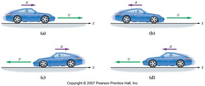
Acceleration

Acceleration (\( a \)) is the rate of change of velocity with respect to time. It can be positive or negative, indicating speeding up or slowing down, respectively.

• Formula:

• SI Unit: meters per second squared (m/s2).

• If velocity and acceleration have the same sign, the object speeds up; if different, it slows down.

Uniform (Constant) Acceleration

When acceleration is constant, the following kinematic equations apply:

These equations allow calculation of unknown variables when three of the five quantities (initial velocity, final velocity, acceleration, time, displacement) are known.

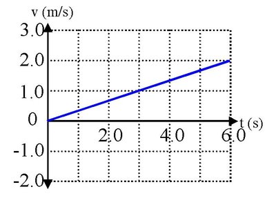
Graphical Analysis of Acceleration

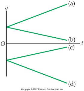
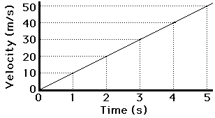
Velocity vs. time graphs with constant acceleration are straight lines; the slope gives acceleration. The area under the velocity-time graph gives displacement.

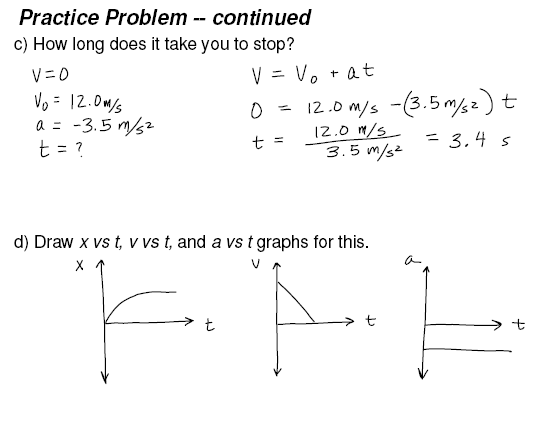
Describing Motion with Graphs

Different types of motion can be represented graphically:

• Constant Velocity: Position vs. time is a straight line; velocity vs. time is horizontal; acceleration vs. time is zero.

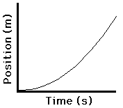
• Constant Acceleration: Position vs. time is a parabola; velocity vs. time is a straight line; acceleration vs. time is horizontal (nonzero).

Practice Problems and Applications

Applying kinematic equations and concepts to real-world scenarios strengthens understanding:

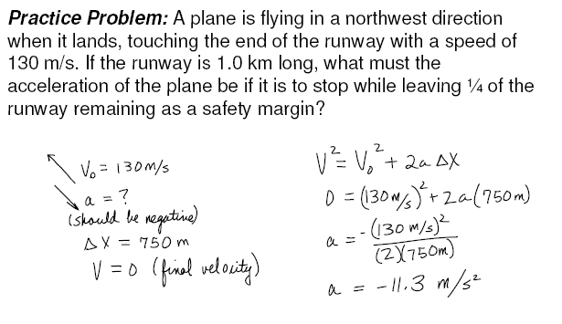
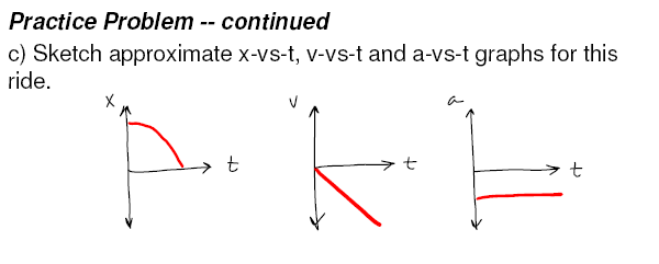
• Stopping Distance: Calculating the required acceleration for a plane to stop on a runway.

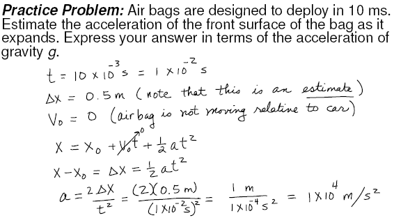
• Airbag Deployment: Estimating the acceleration of an airbag during deployment.

• Reaction Time: Using a meter stick to measure human reaction time.

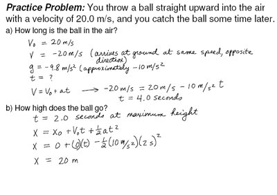
Free Fall

Free fall describes the motion of objects under the influence of gravity alone (ignoring air resistance). The acceleration due to gravity near Earth's surface is downward.

• All objects in free fall experience the same acceleration, regardless of mass.

• Upward motion under gravity is symmetric with downward motion.

Example: Calculating the time a ball spends in the air and its maximum height when thrown upward.

Summary Table: Key Kinematic Quantities

Additional info:

• In free fall, the velocity at which an object returns to its starting point is equal in magnitude and opposite in direction to its initial velocity (if air resistance is neglected).

• Graphical analysis is crucial for interpreting and predicting motion in physics.