Vectors and Static Equilibrium

Introduction to Vectors

Vectors are quantities that have both magnitude and direction. They are essential in physics for representing displacement, velocity, force, and other directional quantities. Understanding how to add, subtract, and resolve vectors is foundational for analyzing physical systems in equilibrium.

Vector Addition

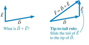
• Tip-to-Tail Rule: To add two vectors, place the tail of the second vector at the tip of the first. The resultant vector is drawn from the tail of the first to the tip of the second.

• Resultant Vector: The sum of two or more vectors is called the resultant vector.

• Commutativity: Vector addition is commutative: \( \vec{A} + \vec{B} = \vec{B} + \vec{A} \).

• Graphical Representation: Vectors are often represented as arrows, with length proportional to magnitude and direction indicating the vector's direction.

Vector Components

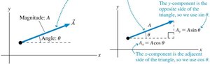
Any vector in a plane can be broken down into two perpendicular components, usually along the x- and y-axes. This process is called resolving a vector into components.

• x-component (\(A_x\)): The projection of the vector along the x-axis.

• y-component (\(A_y\)): The projection of the vector along the y-axis.

• Formulas:

  • \(A_x = A \cos \theta\)

  • \(A_y = A \sin \theta\)

• Magnitude and Direction from Components:

  • \(A = \sqrt{A_x^2 + A_y^2}\)

  • \(\theta = \tan^{-1}(A_y / A_x)\)

Right Triangle Geometry and Trigonometry

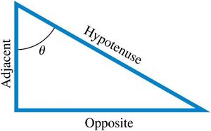
Right triangle relationships are used to relate the sides and angles of vectors resolved into components. The sine, cosine, and tangent functions are defined as ratios of the sides of a right triangle.

• \(\sin \theta = \frac{\text{Opposite}}{\text{Hypotenuse}}\)

• \(\cos \theta = \frac{\text{Adjacent}}{\text{Hypotenuse}}\)

• \(\tan \theta = \frac{\text{Opposite}}{\text{Adjacent}}\)

Static Equilibrium

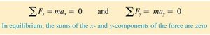
Static equilibrium occurs when an object is at rest and the sum of all forces and torques acting on it is zero. For forces, this means both the x- and y-components must independently sum to zero.

• Equilibrium Conditions:

  • \(\sum F_x = 0\)

  • \(\sum F_y = 0\)

• Free-Body Diagrams (FBDs): Diagrams that show all the forces acting on an object, used to analyze equilibrium situations.

• Applications: Used to solve for unknown forces, such as tensions in ropes or normal forces.

Solving Static Equilibrium Problems with Vector Components

To solve equilibrium problems involving forces at angles, resolve each force into its x- and y-components, then apply the equilibrium conditions to each direction separately.

• Draw a free-body diagram showing all forces.

• Resolve angled forces into components.

• Write equations for \(\sum F_x = 0\) and \(\sum F_y = 0\).

• Solve the system of equations for unknowns (e.g., tensions, weights).

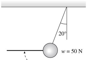
Example: Ball Suspended by Two Ropes

A ball weighing 50 N is suspended by two ropes, one making a 20° angle with the vertical. To find the tensions in the ropes, resolve the forces and apply equilibrium conditions.

• Let \(T_1\) be the tension in the angled rope, \(T_2\) in the horizontal rope, and \(w = 50\) N the weight.

• Vertical equilibrium: \(T_1 \cos 20^\circ = w\)

• Horizontal equilibrium: \(T_1 \sin 20^\circ = T_2\)

• Solve for \(T_1\) and \(T_2\):

  • \(T_1 = \frac{w}{\cos 20^\circ}\)

  • \(T_2 = T_1 \sin 20^\circ\)

Summary Table: Vector and Equilibrium Relationships

Key Takeaways

• Vectors can be added graphically or by components.

• Resolving forces into components simplifies equilibrium analysis.

• Static equilibrium requires the sum of all forces in each direction to be zero.

• Free-body diagrams are essential tools for visualizing and solving equilibrium problems.