Parametric and Vector-Valued Functions

Parametric Curves and Equations

Parametric equations are a fundamental tool in precalculus for describing curves by expressing both x and y as functions of a third variable, typically t (the parameter). This approach allows for more flexible modeling of motion and geometric shapes.

• Parametric Curve: The set of ordered pairs (x, y) where x = f(t) and y = g(t) for t in interval I.

• Parameter: The variable t, which determines the position on the curve.

• Parameter Interval: The set of t values over which the functions are defined.

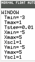
Example: Graphing a Parametric Function

• Given parametric equations, graph the curve by plotting (x(t), y(t)) for t in the interval.

• Calculator window settings are important for visualizing the curve.

Vector-Valued Functions

Vector-valued functions generalize parametric equations by representing position as a vector.

• Definition: A vector-valued function is written as where x(t) and y(t) are functions of t.

• Magnitude: The distance from the origin at time t is

Eliminating the Parameter

Converting Parametric Equations to Cartesian Form

Eliminating the parameter t allows us to rewrite parametric equations as a single equation in x and y, often revealing familiar geometric shapes.

• Method: Solve one equation for t, substitute into the other.

• Result: The resulting equation describes the curve in Cartesian coordinates.

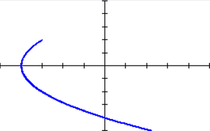
Example: Parabola from Parametric Equations

• After elimination, the graph is a parabola opening to the left with vertex at (5, 0).

Example: Line from Parametric Equations

• Elimination yields a linear equation with slope 2 and y-intercept.

Modeling Planar Motion with Parametric Functions

Simulating Horizontal Motion

Parametric equations are used to model the motion of objects along a path, such as a person walking along a line.

• Position Function: x(t) gives the horizontal position at time t.

• Direction Change: By analyzing x(t), we can estimate when the object changes direction.

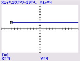
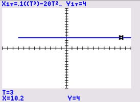
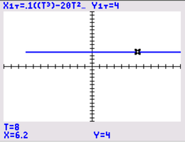
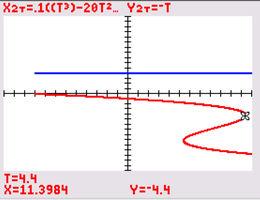
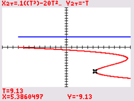
Example: Julia's Walk

• At t = 0, Julia is at x = -9.

• At t = 3, Julia is at x = 10.2.

• At t = 8, Julia is at x = 6.2.

• Julia changes direction at t ≈ 4.4 sec and again at t ≈ 9.13 sec.

Modeling Projectile Motion: Hitting a Baseball

Parametric equations are used to model the path of a projectile, such as a baseball.

• Initial Conditions: Height, velocity, angle, and distance to fence.

• Equations: where is initial velocity, is launch angle, is initial height.

• Analysis: Determine if the ball clears the fence by evaluating y at the x-distance of the fence.

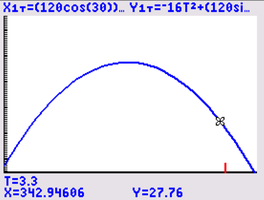
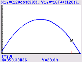
Example: Baseball Path and Fence

• At t = 3.3 sec, x ≈ 343 ft, y ≈ 27.76 ft.

• At t = 3.4 sec, x ≈ 353 ft, y ≈ 23.04 ft.

• The ball does not clear the 30 ft fence at 350 ft; it will hit the wall.

Implicit and Explicit Functions

Implicitly Defined Functions

An equation in two variables may define a function implicitly, even if it is not solved for y in terms of x.

• Implicit Form: Standard form of a line, .

• Explicit Form: Slope-intercept form, , or point-slope form, .

• Advantage: Explicit form directly defines the dependent variable and is suitable for graphing calculators.

Example: Using Implicitly Defined Functions

• Given a relation, solve for y to obtain the explicit function.

Rates of Change for Parametric Curves

Average Rate of Change

For curves defined parametrically, the average rate of change can be computed for x and y independently, and for the curve as a whole.

• Formula:

• Interpretation: The slope between two points on the curve corresponds to the average rate of change.

Example: Parametric Rate of Change

• On interval [0, 2], compute the change in y and x to find the average rate.

• On interval [2, 0], y decreases by an average of 1 unit per unit change in x.

Summary Table: Parametric vs. Explicit vs. Implicit Functions

Additional info: Academic context was added to clarify definitions, formulas, and applications, and to ensure completeness for exam preparation.