Polynomial Functions and Their Graphs

Definition of a Polynomial Function

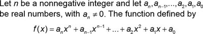
A polynomial function is an expression of the form:

• Where n is a nonnegative integer, and .

• The coefficient is called the leading coefficient.

Characteristics of Polynomial Graphs

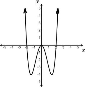
Graphs of polynomial functions of degree 2 or higher are smooth (no sharp corners) and continuous (no breaks).

• They can be drawn without lifting your pencil.

• Degree determines the general shape and number of turning points.

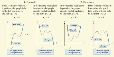
End Behavior of Polynomial Functions

The end behavior describes how the graph behaves as approaches positive or negative infinity. It is determined by the degree and leading coefficient.

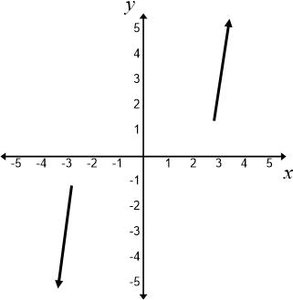
• For odd degree polynomials:

  • If leading coefficient , graph falls left and rises right.

  • If leading coefficient , graph rises left and falls right.

• For even degree polynomials:

  • If leading coefficient , graph rises both left and right.

  • If leading coefficient , graph falls both left and right.

Finding Zeros of Polynomial Functions

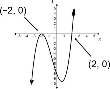
The zeros (or roots) of a polynomial function are the values of for which . These correspond to the x-intercepts of the graph.

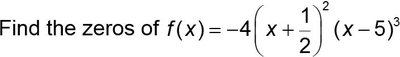
• To find zeros, set and solve for .

• Factoring is often used to solve polynomial equations.

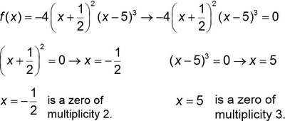
Multiplicity of Zeros

The multiplicity of a zero refers to how many times a particular root occurs. The behavior of the graph at each zero depends on its multiplicity:

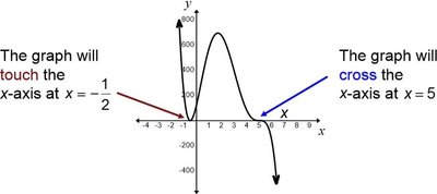
• If the zero has even multiplicity, the graph touches the x-axis and turns around.

• If the zero has odd multiplicity, the graph crosses the x-axis.

• Graphs flatten out near zeros with multiplicity greater than one.

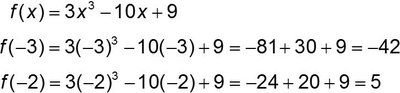
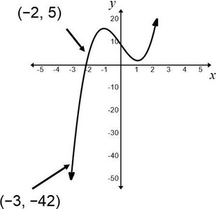
The Intermediate Value Theorem

The Intermediate Value Theorem states: If and have opposite signs for a polynomial function , then there is at least one value between and for which .

• This guarantees the existence of a real root between and .

Turning Points of Polynomial Functions

A turning point is where the graph changes direction from increasing to decreasing or vice versa. For a polynomial of degree , the graph has at most turning points.

• Turning points are related to the degree of the polynomial.

Strategy for Graphing Polynomial Functions

To graph a polynomial function, follow these steps:

1. Determine end behavior using the Leading Coefficient Test.

2. Find x-intercepts (zeros) by solving .

3. Find the y-intercept by computing .

4. Check for symmetry:

   • Y-axis symmetry:

   • Origin symmetry:

5. Check the number of turning points (should not exceed ).

Example: Graphing a Polynomial Function

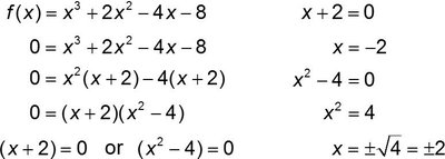
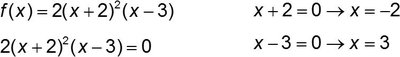
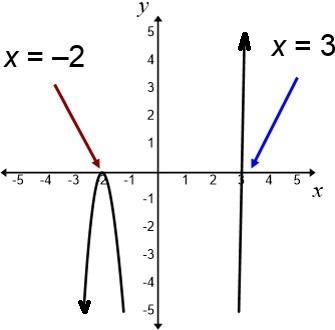
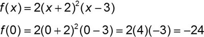
Consider .

• Step 1: End behavior: Degree is 3 (odd), leading coefficient is 2 (positive). Graph rises right, falls left.

• Step 2: Find zeros: (multiplicity 2), (multiplicity 1).

• Step 3: Find y-intercept: .

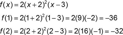
• Step 4: Evaluate at other points for scaling: , .

• Step 5: Check symmetry: No y-axis or origin symmetry.

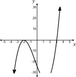
• Step 6: Draw the graph using all information.

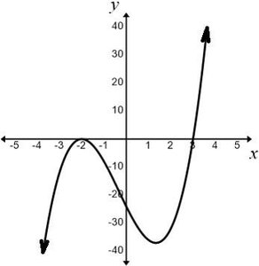
• Step 7: Check turning points: Degree is 3, maximum turning points is 2. The graph has 2 turning points.

Summary Table: End Behavior of Polynomial Functions

Key Formulas

• General polynomial:

• Factoring to find zeros:

Example Applications

• Graphing polynomials to analyze real-world phenomena such as projectile motion, population growth, and economics.

• Using the Intermediate Value Theorem to estimate roots in engineering and science.