Chapter 1: Functions and Graphs

Section 1.1: Graphs and Graphing Utilities

This section introduces the rectangular coordinate system, plotting points, graphing equations, and interpreting graphs using graphing utilities.

• Rectangular Coordinate System: Consists of a horizontal x-axis and a vertical y-axis intersecting at the origin (0,0). Positive numbers are to the right/above the origin; negative numbers are to the left/below.

• Plotting Points: Each point is an ordered pair (x, y). The x-coordinate is the horizontal distance from the origin; the y-coordinate is the vertical distance.

• Example: To plot (−2, 4), move 2 units left and 4 units up from the origin.

• Graphing Equations: The graph of an equation in two variables is the set of all points (x, y) that satisfy the equation.

• Point-Plotting Method: Select values for x, compute corresponding y values, plot the points, and connect them.

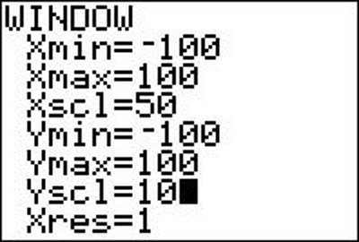
• Graphing Utilities: Graphing calculators and software allow for visualization of equations. The viewing rectangle sets the visible range for x and y values.

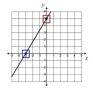
• Intercepts: x-intercept is where the graph crosses the x-axis (y=0); y-intercept is where it crosses the y-axis (x=0).

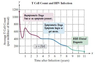
• Interpreting Graphs: Graphs can model real-world data, such as divorce rates or population growth.

Section 1.2: Basics of Functions and Their Graphs

This section covers the definition of relations and functions, function notation, evaluation, and graphical analysis.

• Relation: Any set of ordered pairs. The domain is the set of all first components (x-values); the range is the set of all second components (y-values).

• Function: A relation where each element in the domain corresponds to exactly one element in the range.

• Determining Functions: If an equation gives more than one y for a given x, it is not a function.

• Function Notation: f(x) denotes the value of the function f at x.

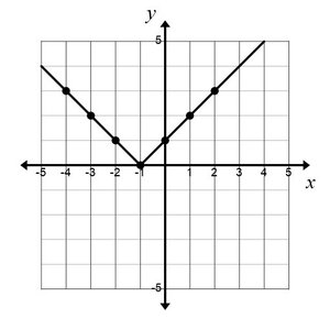
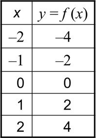
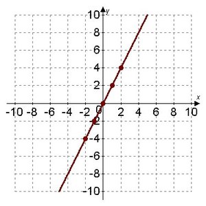
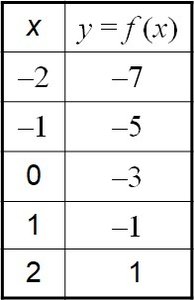
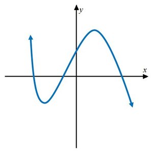
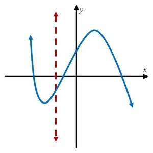
• Graphing Functions: The graph of a function is the set of all ordered pairs (x, f(x)).

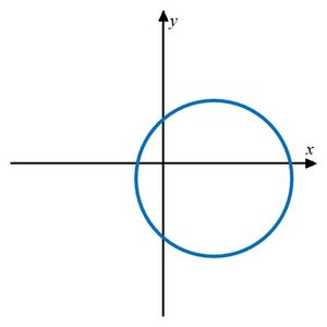
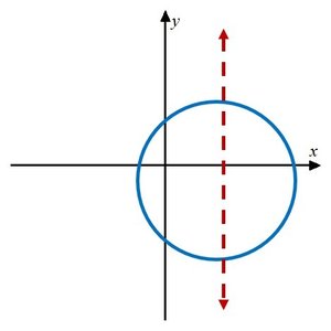
• Vertical Line Test: If any vertical line crosses a graph more than once, it is not a function.

• Domain and Range from Graphs: The domain is the set of all x-values with points on the graph; the range is the set of all y-values.

• Intercepts from Graphs: x-intercepts are where the graph crosses the x-axis; the y-intercept is where it crosses the y-axis.

Section 1.3: More on Functions and Their Graphs

This section explores increasing/decreasing intervals, relative extrema, symmetry, even/odd functions, piecewise functions, and the difference quotient.

• Increasing/Decreasing/Constant: A function is increasing on an interval if f(x) rises as x increases, decreasing if f(x) falls, and constant if f(x) remains unchanged.

• Relative Maximum/Minimum: A relative maximum is a point where f(x) is higher than nearby values; a relative minimum is lower than nearby values.

• Symmetry: Test for symmetry about the y-axis (even), x-axis, or origin (odd).

• Even Function: f(−x) = f(x) for all x in the domain (symmetric about the y-axis).

• Odd Function: f(−x) = −f(x) for all x in the domain (symmetric about the origin).

• Piecewise Function: Defined by different expressions over different intervals.

• Difference Quotient: for ; fundamental in calculus for defining derivatives.

Section 1.4: Linear Functions and Slope

This section covers the concept of slope, forms of linear equations, and graphing lines.

• Slope: The slope m of a line through points and is , .

• Point-Slope Form:

• Slope-Intercept Form:

• Horizontal Line: (slope 0)

• Vertical Line: (undefined slope)

• General Form:

• Graphing Using Intercepts: Find x- and y-intercepts, plot, and draw the line.

• Modeling with Linear Functions: Use data points to find the equation of a line modeling real-world relationships.

Section 1.5: More on Slope

This section discusses parallel and perpendicular lines, interpreting slope as rate of change, and average rate of change.

• Parallel Lines: Nonvertical lines are parallel if they have the same slope.

• Perpendicular Lines: Nonvertical lines are perpendicular if the product of their slopes is −1.

• Slope as Rate of Change: In a linear function, the slope represents the rate at which the dependent variable changes per unit increase in the independent variable.

• Average Rate of Change: For from to , .

Section 1.6: Transformations of Functions

This section covers vertical and horizontal shifts, reflections, stretching/shrinking, and sequences of transformations.

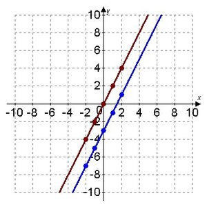
• Vertical Shift: shifts up by c; shifts down by c.

• Horizontal Shift: shifts left by c; shifts right by c.

• Reflections: reflects about the x-axis; reflects about the y-axis.

• Vertical Stretch/Shrink: stretches if , shrinks if .

• Horizontal Stretch/Shrink: shrinks if , stretches if .

• Sequence of Transformations: Apply multiple transformations in order.

Section 1.7: Combinations of Functions; Composite Functions

This section introduces the algebra of functions and composite functions.

• Domain of a Function: The set of all real numbers for which is defined (excluding division by zero and even roots of negatives).

• Algebra of Functions:

  • Sum:

  • Difference:

  • Product:

  • Quotient: ,

• Composite Function: . The domain is all x in the domain of g such that is in the domain of f.

• Writing Functions as Compositions: Express a function as the composition of two or more functions.

Section 1.8: Inverse Functions

This section defines inverse functions, how to find them, and their graphical properties.

• Inverse Function: is the inverse of f if and .

• Finding the Inverse: Replace with y, interchange x and y, solve for y, and relabel as .

• Horizontal Line Test: A function has an inverse that is also a function if no horizontal line crosses its graph more than once.

• Graph of Inverse: The graph of is a reflection of the graph of f about the line .

Section 1.9: Distance and Midpoint Formulas; Circles

This section provides formulas for distance and midpoint between points, and the equation of a circle.

• Distance Formula: The distance between and is .

• Midpoint Formula: The midpoint is .

• Circle: The set of all points equidistant from a center (h, k). Standard form: .

• General Form: ; can be converted to standard form by completing the square.

Section 1.10: Modeling with Functions

This section demonstrates how to construct mathematical models from verbal descriptions and formulas.

• Constructing Functions: Translate real-world scenarios into mathematical functions, such as cost, revenue, or geometric models.

• Example: Cost functions for two shops: , .

• Geometric Modeling: Express volume or area as a function of a variable, considering constraints on the domain.

Additional info: These notes are based on the content of Chapter 1 from a standard Precalculus textbook and are suitable for college-level precalculus students preparing for exams or reviewing foundational concepts in functions and graphs.